Application of normal mode functions for the (g) 10 days improved - PowerPoint PPT Presentation
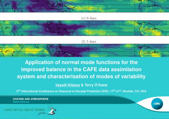
(e) 0 days (f) 5 days Application of normal mode functions for the (g) 10 days improved balance in the CAFE data assimilation system and characterisation of modes of variability Vassili Kitsios & Terry OKane (h) 15 days 2 nd
(e) 0 days (f) 5 days Application of normal mode functions for the (g) 10 days improved balance in the CAFE data assimilation system and characterisation of modes of variability Vassili Kitsios & Terry O’Kane (h) 15 days 2 nd International Conference on Seasonal to Decadal Prediction (S2D), 17 th -21 st , Boulder, CO, USA OCEANS AND ATMOSPHERE www.csiro.au CSIRO (i) 20 days
Approach • Will focus on the characterisation of the Madden Julian Oscillation (MJO) via a Normal Mode Functions (NMF) decomposition of JRA55, and dis- cuss implications for Normal Mode Inialisation (NMI) . • MJO is a mode of variability resulting from coupled tropical deep convec- tion and atmospheric dynamics. • Use key MJO properties to identify representatives NMFs: – Eastward propagating – Dominant variance over intra-seasonal timescales: 30-90 days. – Tropics centric dynamics. – Horizontal velocity field has a dominant longitudinal wave of k = 1 . – Dominant component of the zonal velocity is symmetric about the equator. • Using one such mode we produce phase and conditional averages of: – velocity potential to illustrate atmospheric dynamics – outgoing longwave radiation to illustrate convection • Acknowledge ˇ Zagar for sharing the NCAR NMF code, MODES . Application of normal mode functions for the improved balance in the CAFE data assimilation system and characterisation of modes of variability
What are Normal Mode Functions ? • Decompose 3D ( λ, φ, σ ) velocity ( u, v ) and geopotential height ( h ) fields into horizonal and vertical scales , and mode type , using the eigensolu- tion of the linearised primitive equations on a sphere. • Each scale decomposed into: Balanced Component ( BAL ) ; Eastward Inertial Gravity Wave ( EIG ) ; Westward Inertial Gravity Wave ( WIG ). • Vertical Structure Functions (VSF), G m in σ coordinates. • Longitudinal ( λ ) waves e i kλ • Meridional ( φ ) Horizonal Structure Functions (HSF) of wind and height ( U, V, H ) for EIG, WIG and BAL modes. � √ gD m � u ( σ, λ, φ, t ) � M 0 0 � K √ gD m � � e i kλ v ( σ, λ, φ, t ) = G m ( σ ) 0 0 h ( σ, λ, φ, t ) 0 0 gD m m =1 k = − K � p U ( φ ) N � EIG,WIG,BAL χ p � � − i V ( φ ) knm ( t ) H ( φ ) p n =0 knm • Complex coefficients, χ p knm ( t ) , represent contributions of each compo- Application of normal mode functions for the improved balance in the CAFE data assimilation system and characterisation of modes of variability nent.
Vertical Structure Functions • VSF given by solution of the VSF eigenvalue problem (EVP). • VSF EVP requires only a time and horizontally averaged static stability profile in σ coordinates. • Equivalent heights D m (eigenvalues) are indicative of vertical scale. • VSF G m ( σ ) (eigenvectors) have m − 1 zero crossings. G 1 is the barotropic, G 2 the first baroclinic, G 3 the second baroclinic, ... • For large m , the VSF represent boundary layer processes. (a) static stability ≡ Γ 0 (b) equivalent height ≡ D m (c) vertical structure functions 10 4 10 0 10 0 10 3 m=1 10 2 σ × p 0 [hPa] D m [metres] σ × p 0 [hPa] 10 1 10 1 m=2 m=8 10 1 m=15 m=28 10 2 10 2 10 0 10 − 1 10 3 10 3 10 1 10 2 10 3 10 4 10 5 0 10 20 30 40 − 0 . 5 0 . 0 0 . 5 Γ 0 [K] vertical mode number amplitude [unitless] Application of normal mode functions for the improved balance in the CAFE data assimilation system and characterisation of modes of variability
Horizontal Structure Functions • HSF given by solution of a HSF EVP for each equivalent height ( D m ). • Eigenvectors give meridional dependence, with mode types (EIG, WIG, BAL) defined by symmetry properties. • Frequency ν (eigenvalue) is indicative of temporal scale. (c) U q knm ( φ ) (a) timescales for m = 28 (b) timescales 10 4 10 3 BAL BAL (1 , 1 ,m ) EIG (1 , 0 , 28) 75 EIG WIG (1 , 0 ,m ) EIG (1 , 0 , 8) WIG 10 3 EIG (1 , 0 ,m ) 50 BAL (1 , 1 , 15) MRG 90days 10 2 KW BAL (1 , 1 , 8) 25 knm [days] knm [days] 60days latitude ( φ ) 10 2 30days 0 1 /ν q 1 /ν q 10 1 10 1 − 25 − 50 10 0 10 0 − 75 − 30 − 20 − 10 0 10 20 30 0 10 20 30 40 − 1 0 1 longitudinal wavenumber (k) vertical mode number (m) amplitude • Recall for MJO: k = 1 ; tropics centric; U is symmetric • Only the EIG n = 0 , WIG n = 0 , and BAL n = 1 are tropics centric with the appropriate symmetries. • EIG m = 23 − 32 ; BAL m = 11 − 22 have intra-seasonal timescales. Application of normal mode functions for the improved balance in the CAFE data assimilation system and characterisation of modes of variability
Energy Contribution χ p knm ( t ) χ p ∗ knm ( t ) of NMFs in JRA55 • BAL dominates for low k , IG dominate for high k • BAL dominates for all vertical modes m • For ( k, n ) = (1 , 1) BAL HSF eigenvectors have MJO-like properties: – BAL ( k, n, m ) = (1 , 1 , 2) and (1 , 1 , 2) local peaks in energy, but too fast – BAL ( k, n, m ) = (1 , 1 , 15) has HSF eigenvalue of 46 days. • For ( k, n ) = (1 , 0) EIG HSF eigenvectors also have MJO-like properties: – EIG ( k, n, m ) = (1 , 0 , 8) has most energy, but timescale too fast – EIG ( k, n, m ) = (1 , 0 , 28) has HSF eigenvalue of 56 days. (a) (b) (c) ( k, n ) = (1 , 1) (d) ( k, n ) = (1 , 0) 10 4 BAL 10 3 EIG WIG 10 2 nonzonal energy [J/kg] total 10 1 10 0 10 − 1 10 − 2 10 − 3 10 − 4 Application of normal mode functions for the improved balance in the CAFE data assimilation system and characterisation of modes of variability 10 0 10 1 10 2 0 10 20 30 0 10 20 30 0 10 20 30 vertical mode (m) zonal wavenumber (k) vertical mode (m) vertical mode (m)
Cross-spectral Analysis of Candidate NMFs • All candidate modes are tropics centric and have the appropriate symme- tries. • Only EIG ( k, n, m ) = (1 , 0 , 28) has an intra-seasonal timescale, and propagates eastward, but has low energy. • Cross-spectral analysis identifies only slow intra-seasonal timescales are coherent between EIG ( k, n, m ) = (1 , 0 , 28) and the more energetic modes. • Fast Kelvin wave removed from energetic EIG ( k, n, m ) = (1 , 0 , 8) . (a) PSD of EIG ( k, 0 , 8) [J/kg] (b) PSD of EIG ( k, 0 , 28) [J/kg] (c) coherence (d) coherence output [J/kg] 0 . 5 1 . 0 10 1 10 1 10 − 1 0 . 4 0 . 8 10 0 10 0 10 − 2 0 . 3 0 . 6 f [1/days] 10 − 1 10 − 1 0 . 2 0 . 4 10 − 3 10 − 2 10 − 2 0 . 1 0 . 2 10 − 3 10 − 3 30days 10 − 4 10 − 4 10 − 4 0 . 0 0 . 0 2 4 6 8 10 2 4 6 8 10 2 4 6 8 10 2 4 6 8 10 k k k k Application of normal mode functions for the improved balance in the CAFE data assimilation system and characterisation of modes of variability
Cross-spectral Analysis of Candidate NMFs • All candidate modes are tropics centric and have the appropriate symme- tries. • Only EIG ( k, n, m ) = (1 , 0 , 28) has an intra-seasonal timescale, and propagates eastward, but has low energy. • Cross-spectral analysis identifies only slow intra-seasonal timescales are coherent between EIG ( k, n, m ) = (1 , 0 , 28) and the more energetic modes. • Repeated for all vertical scales ( m ) with k = 1 for BAL and EIG. k k k k (e) coherence output of EIG (1 , 0 ,m ) [J/kg] (f) coherence output of BAL (1 , 1 ,m ) [J/kg] 10 2 0 . 5 10 2 10 1 10 1 0 . 4 10 0 10 0 0 . 3 f [1/days] 10 − 1 10 − 1 0 . 2 10 − 2 10 − 2 0 . 1 10 − 3 10 − 3 10 − 4 10 − 4 0 . 0 5 10 15 20 25 30 35 5 10 15 20 25 30 35 m m • Other candidate modes highlighted in coherence output clusters. Application of normal mode functions for the improved balance in the CAFE data assimilation system and characterisation of modes of variability
Phase Average on Basis of EIG ( k, n, m ) = (1 , 0 , 28) • Phase angle calculated from complex χ p nmk . Dates associated with each phase angle octant averaged. All modes contribute to phase averages. • Velocity potential is a propagating longitudinal wave, with a vertical sign change representing upper level divergence and lower level convergence. Application of normal mode functions for the improved balance in the CAFE data assimilation system and characterisation of modes of variability
Phase Average on Basis of EIG ( k, n, m ) = (1 , 0 , 28) • Phase angle calculated from complex χ p nmk . Dates associated with each phase angle octant averaged. All modes contribute to phase averages. • OLR has a dipole pattern over the maritime continent, tracking with veloc- ity potential of like sign. Application of normal mode functions for the improved balance in the CAFE data assimilation system and characterisation of modes of variability
Large and Persistent MJO Events • Start and end of each event defined as discontinuities in phase angle of EIG ( k, n, m ) = (1 , 0 , 28) . • Persistent events have a continuous phase for longer than 270 ◦ . • Large events have a magnitude in the upper quartile. • Composite average magnitude is greater than background for 20 days be- fore and after day 0 . • Composite average phase angle indicates eastward propagation. • Dates associated with each phase shift identified and averaged to produce composite fields of velocity potential and outgoing longwave radiation. Application of normal mode functions for the improved balance in the CAFE data assimilation system and characterisation of modes of variability
Recommend
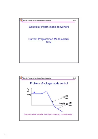


![1 [9-4] Mor M. Peretz, Switch-Mode Power Supplies Current feedback loop I o L i o V o v o S V](https://c.sambuz.com/1071065/1-s.webp)


More recommend
Explore More Topics
Stay informed with curated content and fresh updates.