Application of Inverse Methods to Problems from Systems Biology - PowerPoint PPT Presentation
Application of Inverse Methods to Problems from Systems Biology Peter Schuster Institut fr Theoretische Chemie, Universitt Wien, Austria and The Santa Fe Institute, Santa Fe, New Mexico, USA Inverse Problems: Computational Methods an
Application of Inverse Methods to Problems from Systems Biology Peter Schuster Institut für Theoretische Chemie, Universität Wien, Austria and The Santa Fe Institute, Santa Fe, New Mexico, USA Inverse Problems: Computational Methods an Emerging Applications UCLA Conference Center at Lake Arrowhead, 11.– 16.06.2006
Web-Page for further information: http://www.tbi.univie.ac.at/~pks
1. What is systems biology ? 2. Forward and inverse problems in modeling 3. Three examples 4. Bifurcation analysis of gene regulation 5. Analysis of a synthetic oscillator
1. What is systems biology ? 2. Forward and inverse problems in modeling 3. Three examples 4. Bifurcation analysis of gene regulation 5. Analysis of a synthetic oscillator
From qualitative data to quantitative modeling Genomics, proteomics, interactomics Metabolomics, functional genomics Systems biology (quantitative biology)
time Analysis by gel electrophoresis Jeff Rogers, Gerald F. Joyce. RNA 7 :395-404, 2001
The same section of the microarray is shown in three independent hybridizations. Marked spots refer to: (1) protein disulfide isomerase related protein P5, (2) IL-8 precursor, (3) EST AA057170, and (4) vascular endothelial growth factor. Gene expression DNA microarray representing 8613 human genes used to study transcription in the response of human fibroblasts to serum. V.R.Iyer et al ., Science 283 : 83-87, 1999
A pH-modulated, self-replicating peptide Shao Yao, Indraneel Ghosh, Reena Zutshi, Jean Chmielewski. J.Am Chem.Soc. 119 :10559-10560, 1997
Stoichiometric equations A + B � X 2 X � Y Y + X � D SBML – systems biology markup language d d a b = = − k a b 1 Kinetic differential equations d t d t d x = − 2 − k a b k x k x y 1 2 3 d t ODE Integration d y = 2 − k x k x y 2 3 d t d d Solution curves = x i (t) k x y 3 d t Concentration The elements of the simulation tool MiniCellSim t SBML : Bioinformatics 19 :524-531, 2003; Time CVODE : Computers in Physics 10 :138-143, 1996
A model genome with 12 genes 1 2 3 4 5 6 7 8 9 10 11 12 Regulatory protein or RNA Regulatory gene Enzyme Structural gene Metabolite Sketch of a genetic and metabolic network
A B C D E F G H I J K L Biochemical Pathways 1 2 3 4 5 6 7 8 9 10 The reaction network of cellular metabolism published by Boehringer-Ingelheim.
The citric acid or Krebs cycle (enlarged from previous slide).
4×10 6 Nucleotides E. coli : Length of the Genome Number of Cell Types 1 Number of Genes 4 290 3×10 9 Nucleotides Man : Length of the Genome Number of Cell Types 200 Number of Genes 30 000 - 60 000
The bacteriophage � lysis/lysogeny decision circuit. A. Arkin, J. Ross, H.H. McAdams. Genetics 149 :1633-1648, 1998.
Elimination of introns through splicing genomic DNA mRNA AAA The gene is a stretch of DNA which after transcription and processing gives rise to a mRNA
Sex determination in Drosophila through alternative splicing The process of protein synthesis and its regulation is now understood but the notion of the gene as a stretch of DNA has become obscure. The gene is essentially associated with the sequence of unmodified amino acids in a protein, and it is determined by the nucleotide sequence as well as the dynamics of the the process eventually leading to the m-RNA that is translated.
The difficulty defining the gene Helen Pearson, Nature 441 : 399-401, 2006
Stefan Bornholdt. Less is more in modeling large genetic networks. Science 310 , 449-450 (2005)
1. What is systems biology ? 2. Forward and inverse problems in modeling 3. Three examples 4. Bifurcation analysis of gene regulation 5. Analysis of a synthetic oscillator
Kinetic differential equations d x = = = ( ; ) ; ( , , ) ; ( , , ) K K f x k x x x k k k 1 1 n m d t Reaction diffusion equations ∂ x = ∇ + 2 ( ; ) Solution curves : ( ) D x f x k x t ∂ t x i (t) Concentration Parameter set = ( T , p , p H , I , ) ; j 1 , 2 , , m K K k j General conditions : T , p , pH , I , ... t ( 0 ) Initial conditions : x Time Boundary conditions : � boundary ... S , normal unit vector ... u x S = Dirichlet : ( , ) g r t ∂ S = x = ⋅ ∇ ˆ Neumann : ( , ) u x g r t ∂ u The forward problem of chemical reaction kinetics (Level I)
Kinetic differential equations d x = = = ( ; ) ; ( , , ) ; ( , , ) K K f x k x x x k k k 1 1 n m d t Reaction diffusion equations ∂ x 2 = ∇ + Genome: Sequence I G ( ; ) Solution curves : ( ) D x f x k x t ∂ t x i (t) Concentration Parameter set = ( G I ; , , , , ) ; 1 , 2 , , K K k j T p p H I j m General conditions : T , p , pH , I , ... t ( 0 ) Initial conditions : x Time Boundary conditions : boundary ... S , normal unit vector � ... u x S = Dirichlet : ( , ) g r t ∂ S = x = ⋅ ∇ ˆ ( , ) Neumann : u x g r t ∂ u The forward problem of biochemical reaction kinetics (Level I)
Kinetic differential equations d x = = = ( ; ) ; ( , , ) ; ( , , ) K K f x k x x x k k k 1 1 n m d t Reaction diffusion equations ∂ x = ∇ + 2 ( ; ) D x f x k ∂ t General conditions : T , p , pH , I , ... ( 0 ) Initial conditions : x Genome: Sequence I G Boundary conditions : boundary ... S , normal unit vector � ... u Parameter set x S = = Dirichlet : ( , ) ( G I ; , , , , ) ; 1 , 2 , , g r t K K k j T p p H I j m ∂ S = x = ⋅ ∇ Neumann : ˆ ( , ) u x g r t ∂ u Data from measurements (t ); = 1, 2, ... , x j N j x i (t ) j Concentration The inverse problem of biochemical t Time reaction kinetics (Level I)
Kinetic differential equations d x = = = f ( ; ) ; ( , K , ) ; ( , K , ) x k x x x k k k 1 1 n m d t Bifurcation analysis Reaction diffusion equations � ( , ; ) ∂ k k j k i x = ∇ + 2 f ( ; ) Genome: Sequence I G D x x k ∂ t k i P x n P Parameter set x n P x m = ( G I ; , , , , ) ; 1 , 2 , , K K k j T p p H I j m x m ( ) x t General conditions : T , p , pH , I , ... P time ( 0 ) Initial conditions : x x n x m k j Boundary conditions : boundary ... S , normal unit vector � ... u x S = Dirichlet : ( , ) g r t ∂ S = x = ⋅ ∇ ˆ Neumann : ( , ) u x g r t ∂ u The forward problem of bifurcation analysis (Level II)
Kinetic differential equations d x = = = ( ; ) ; ( , , ) ; ( , , ) K K f x k x x x k k k 1 1 n m d t Reaction diffusion equations ∂ x = ∇ + 2 ( ; ) D x f x k ∂ t General conditions : T , p , pH , I , ... ( 0 ) Initial conditions : x Genome: Sequence I G Boundary conditions : boundary ... S , normal unit vector � ... u Parameter set x S = Dirichlet : = ( , ) ( G I ; , , , , ) ; 1 , 2 , , g r t K K k j T p p H I j m ∂ S = x = ⋅ ∇ Neumann : ˆ ( , ) u x g r t ∂ u Bifurcation pattern � ( , ; ) k k j k k 2 i P 1 x n P 2 x P x m x The inverse problem of bifurcation P x k 1 analysis (Level II) x
Stock Solution [A] = a Reaction Mixture [A],[X] 0 r * A k 1 A X X A A A X A A k 2 A X A X k 3 A A +2 3 X A X X k 4 A A � R- A r X 1 Flow rate = A r A A 0 A X A X A X r 0 X X X X A A
0.5 � r Stationary concentration x Thermodynamic 0.4 branch 0.3 0.2 Bistability r cr,1 r cr,2 0.1 0.02 0.04 0.06 0.08 0.10 0.12 0.14 Flow rate r
r Kinetic differential equations: * A d [ A ] d a = = − − + 2 + + 2 ( ) ( ) ( ) r a a k k x a k k x x 0 1 3 2 4 d t d t k 1 d [ X ] d x A X = = − + + − + 2 2 ( ) ( ) r x k k x a k k x x 1 3 2 4 k 2 d t d t k 3 +2 3 A X X k 4 r 0 A r 0 X
r Kinetic differential equations: * A d [ A ] d a = = − − + 2 + + 2 ( ) ( ) ( ) r a a k k x a k k x x 0 1 3 2 4 d t d t k 1 d [ X ] d x A X = = − + + − + 2 2 ( ) ( ) r x k k x a k k x x 1 3 2 4 k 2 d t d t k 3 Steady states: +2 3 A X X + − + + + − = 3 2 k 4 ( ) ( ) 0 x k k x k a x k k r k a 3 4 3 0 1 2 1 0 r 0 A r 0 X
r Kinetic differential equations: * A d [ A ] d a = = − − + 2 + + 2 ( ) ( ) ( ) r a a k k x a k k x x 0 1 3 2 4 d t d t k 1 d [ X ] d x A X = = − + + − + 2 2 ( ) ( ) r x k k x a k k x x 1 3 2 4 k 2 d t d t k 3 Steady states: +2 3 A X X + − + + + − = 3 2 k 4 ( ) ( ) 0 x k k x k a x k k r k a 3 4 3 0 1 2 1 0 r = = α = = − + + α − α = 3 2 , 1 : 2 ( 2 ) 0 k k k k x x a x r a 0 A 1 2 3 4 0 0 r 0 X
Recommend
More recommend
Explore More Topics
Stay informed with curated content and fresh updates.
