Application of Information or How I learnt to stop Theory to Fault - PowerPoint PPT Presentation

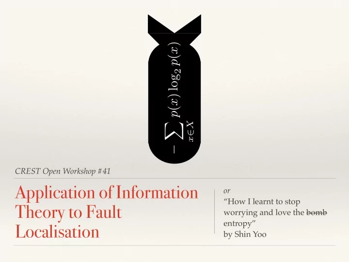
p ( x ) log 2 p ( x ) x ∈ X X ) = − CREST Open Workshop #41 Application of Information or “How I learnt to stop Theory to Fault worrying and love the bomb entropy” Localisation by Shin Yoo

This talk is… ❖ Not a theoretical masterclass on application of Shannon Entropy to software engineering, unfortunately ❖ Rather a story of a clueless software engineer who learnt to appreciate the power of information theory

The Problem Domain ❖ Fault Localisation: given observations from test execution (which includes both passing and failing test cases), identify where the faulty statement lies.

Spectra Based Fault Localisation e p e f − e p + n p + 1 Program Spectrum Formula (Suspiciousness) Higher ranking = Fewer statements to check Tests Ranking

Spectra-Based Fault Localisation Structural Test Test Test Spectrum Tarantula Rank Elements t 1 t 2 t 3 e p e f n p n f 1 0 0 2 0.00 9 s 1 • 1 0 0 2 0.00 9 s 2 • e f 1 0 0 2 0.00 9 s 3 • e f + n f 1 0 0 2 0.00 9 s 4 Tarantula = • e p e f 1 0 0 2 0.00 9 s 5 e p + n p + • e f + n f 1 1 0 1 0.33 4 s 6 • • s 7 (faulty) 0 2 1 0 1.00 1 • • 1 1 0 1 0.33 4 s 8 • • 1 2 0 0 0.50 2 s 9 • • • Result P F F

How do we evaluate these? e p ( Wong 2 = e f − e p Op 2 = e f − − 1 if n f > 0 e p + n p + 1 Op 1 = n p otherwise e f 2 e f e f + n p + 2( e p + n f ) e f + n f + e p e f e f e f + n f e f Tarantula = Jaccard = e p e f e p + n p + e f + n f + e p e f + n f + e p e f + n f 2( e f + n p ) e f + n p e f e p 2( e f + n p ) + e p + n f n f + e p AMPLE = | | − e f + n f e p + n p e f e f Ochiai = p ( e f + n f ) · ( e f + e p ) n f + e p e f + n p e f Wong 1 = e f e f + n f + e p + n p 2 e f e f e f + n f + e p + n p e f + n f 2 e f + n f + e p e f + n p − n f − e p e p e f e p + n p + 1 e f e f e f + n f e f + n f + e p + n p 2( + )  e f + n f e f + e p if e p ≤ 2 e p   Wong 3 = e f − h, h = 2 + 0 . 1( e p − 2) if 2 < e p ≤ 10  2 . 8 + 0 . 001( e p − 10) if e p > 10 

Expense Metric Statement Ranking S Y E ( τ , p, b ) = Ranking of b according to τ B S X Number of statements in p ∗ 100 B S Y F S X F ❖ Assumes that the developer checks the ranking from top to S Y bottom S X A A ❖ The higher the faulty statement is ranked, the earlier the fault is Formula X Formula Y found

Does every test execution help you? ❖ When a statement is executed by a failing test, we suspect it more; by a passing test, we suspect it less. ❖ Ideally , we want the failing test to only execute the faulty statement, which is not possible of course. ❖ Practically , we want the subset of test runs that gives us the most distinguishing power, and we want this as early as possible.

What is the information gain of executing one more test?

τ ( s j | T i ) Convert suspiciousness P T i ( B ( s j )) = P m j =1 τ ( s j | T i ) into probability m Compute the Shannon Entropy X H T i ( S ) = − P T i ( B ( s j )) · log P T i ( B ( s j )) of Fault Locality j =1 P T i +1 ( B ( s j )) = P T i +1 ( B ( s j ) | F ( t i +1 )) · α + Assuming the failure rate observed so far, compute lookahead P P T i +1 ( B ( s j ) |¬ F ( t i +1 )) · (1 − α ) We can predict the information gain of a test case!

sed, v2, F_AG_19 grep, v3, F_KP_3 flex, v5, F_AA_4 flex, v5, F_JR_2 1.0 1.0 1.0 1.0 Suspiciousness Suspiciousness Suspiciousness Suspiciousness 0.5 FLINT FLINT FLINT FLINT TCP TCP TCP TCP Random Random Random Random 10 40 Exp. Reduction FLINT Exp. Reduction FLINT Exp. Reduction FLINT Exp. Reduction FLINT 10 10 Exp. Reduction Greedy Exp. Reduction Greedy Exp. Reduction Greedy Exp. Reduction Greedy Expense Reduction Expense Reduction Expense Reduction Expense Reduction 30 5 0 20 0 0 − 5 10 − 20 − 10 0 − 15 − 20 − 40 − 20 0 0 0 0 20 20 20 20 40 40 40 40 60 60 60 60 80 80 80 80 100 100 100 100 Percentage of Executed Tests Percentage of Executed Tests Percentage of Executed Tests Percentage of Executed Tests

Lessons Learned #1 ❖ Probabilistic view works! Even when there are some wrinkles in your formulations. ❖ Software artefacts tend to exhibit continuity (e.g. coverage of a test case does not change dramatically between versions, etc). This helps the point 1.

Problem Solved…? ❖ Various empirical study established partial rankings between formulas at first. ❖ Then a theoretical study proved the dominance between formulas and their performance in Expense metrics.

But then machines arrived. Aside: we also automatically evolved formulas using GP, which we then proved cannot be bettered by humans. So technically machines arrived twice .

Machine Based Evaluation ❖ Qi et al. took a backward approach ❖ Use suspicious score as weights to mutate program states until Genetic Programming can repair the fault. ❖ The better the localisation, the quicker the repair will be found.

Strange Results ❖ Theory says Jaccard formula is worse than Op2. ❖ But machines found it much easier to repair programs when using the localisation from Jaccard. ❖ Why?

Abstraction destroys Information ❖ Expense metric assumes linear consumption of the result (i.e. < developer checks statements following the ranking). Same ranking, completely different ❖ GP consumes raw amount of information. suspiciousness numbers, which is a much richer source of information.

New Evaluation Metric technique, L , that can always pinpoint s f as follows: ❖ Following the way we ⇢ 1 ( s i = s f ) L ( s i ) = (0 < ✏ ⌧ 1 , s i 2 S, s i 6 = s f ) predicted information yield, ✏ that we can convert outputs of FL techniques that we should be able to describe ⌧ ( s i ) the true fault locality as a P τ ( s i ) = i =1 ⌧ ( s i ) , (1 ≤ i ≤ n ) P n probability distribution. erts suspiciousness scores given by any ❖ Subsequently, measure the ln P L ( s i ) X D KL ( P L || P τ ) = P τ ( s i ) P L ( s i ) cross-entropy between the true i distribution and one generated Locality Information Loss (LIL) by any technique. defined with Kullback-Leibler divergence

Worth a thousand words. Op2 (LIL=7.34) Ochiai (LIL=5.96) Faulty Statement Suspiciousness Suspiciousness 0.8 0.8 0.4 0.4 Faulty Statement 0.0 0.0 Executed Statements Executed Statements Jaccard (LIL=4.92) MUSE (LIL=0.40) Faulty Statement Faulty Statement Suspiciousness Suspiciousness 0.8 0.8 0.4 0.4 0.0 0.0 Executed Statements Executed Statements

Lessons Learned #2 ❖ Entropy measures are much richer than simply counting something: it gives you a holistic view. ❖ Cross-entropy is a vastly underused tool in software engineering in general.

Spectra Based Fault Localisation e p e f − e p + n p + 1 Program Spectrum Formula (Suspiciousness) Higher ranking = Fewer statements to check Tests Ranking

grep, v3, F_KP_3 1.0 Suspiciousness 0.5 FLINT TCP Random Exp. Reduction FLINT 10 Exp. Reduction Greedy Expense Reduction 0 − 10 − 20 0 20 40 60 80 100 Percentage of Executed Tests