Anisotropic Density Estimation in Global Illumination Lars Schjth - PowerPoint PPT Presentation
Introduction Three different density estimators Comparison and evaluation Anisotropic Density Estimation in Global Illumination Lars Schjth University of Copenhagen Department of Computer Science 29. Maj 2009 Introduction Three different
Introduction Three different density estimators Comparison and evaluation Anisotropic Density Estimation in Global Illumination Lars Schjøth University of Copenhagen Department of Computer Science 29. Maj 2009
Introduction Three different density estimators Comparison and evaluation Caustic by reflection
Introduction Three different density estimators Comparison and evaluation Photon distribution
Introduction Three different density estimators Comparison and evaluation Density Estimation
Introduction Three different density estimators Comparison and evaluation Density Estimation
Introduction Three different density estimators Comparison and evaluation Density Estimation
Introduction Three different density estimators Comparison and evaluation Kernel Density Estimation Kernel Denisty Estimator, h = 0.008 8 7 6 5 4 3 2 1 0 −0.6 −0.4 −0.2 0 0.2 0.4 0.6 0.8 1 1.2 � x − x i � n � f ( x ) = 1 � K nh h i = 1
Introduction Three different density estimators Comparison and evaluation Kernel Density Estimation Kernel Denisty Estimator, h = 0.008 Kernel Denisty Estimator, h = 0.04 8 4 7 3.5 6 3 5 2.5 4 2 3 1.5 2 1 1 0.5 0 0 −0.6 −0.4 −0.2 0 0.2 0.4 0.6 0.8 1 1.2 −0.6 −0.4 −0.2 0 0.2 0.4 0.6 0.8 1 1.2 � x − x i � n � f ( x ) = 1 � K nh h i = 1
Introduction Three different density estimators Comparison and evaluation KNN Kernel Estimator KNN Kernel Denisty Estimator, k = 25 12 10 8 6 4 2 0 −0.6 −0.4 −0.2 0 0.2 0.4 0.6 0.8 1 1.2 � x − x i � n � f ( x ) = 1 1 � h ( x ) K n h ( x ) i = 1
Introduction Three different density estimators Comparison and evaluation Variable Kernel Estimator Variable Kernel Denisty Estimator, k = 25 12 10 8 6 4 2 0 −0.6 −0.4 −0.2 0 0.2 0.4 0.6 0.8 1 1.2 � x − x i � n � f ( x ) = 1 1 � h ( x i ) K n h ( x i ) i = 1
Introduction Three different density estimators Comparison and evaluation Mean Integrated Square Error � � � � 2 d x + MISE ( � E � var � f ) = f ( x ) − f ( x ) f ( x ) d x
Introduction Three different density estimators Comparison and evaluation Mean Integrated Square Error � � � � 2 d x + MISE ( � E � var � f ) = f ( x ) − f ( x ) f ( x ) d x � �� � 2 � f ) = 1 AMISE ( � 4 h 4 f ′′ ( x ) 2 dx y 2 K ( y ) dy + ( nh ) − 1 K ( y ) 2 dy
Introduction Three different density estimators Comparison and evaluation Trade-off problem in CG Effect of bandwidth Low High
Introduction Three different density estimators Comparison and evaluation Three radiance estimates Jensen’s radiance estimate k � 1 L r ( x , ω ) ≈ � L r ( x , ω ) = f r ( x , ω i , ω )Φ i π h k ( x ) 2 i = 1
Introduction Three different density estimators Comparison and evaluation Three radiance estimates Jensen’s radiance estimate k � 1 L r ( x , ω ) ≈ � L r ( x , ω ) = f r ( x , ω i , ω )Φ i π h k ( x ) 2 i = 1 Diffusion based radiance estimate � ( x − x i ) T D − 1 ( x − x i ) � n � 1 � L r ( x , � ω ) = f r ( x , � ω )Φ i K ω i , � π h 2 √ h 2 det D i = 1
Introduction Three different density estimators Comparison and evaluation Three radiance estimates Jensen’s radiance estimate k � 1 L r ( x , ω ) ≈ � L r ( x , ω ) = f r ( x , ω i , ω )Φ i π h k ( x ) 2 i = 1 Diffusion based radiance estimate � ( x − x i ) T D − 1 ( x − x i ) � n � 1 � L r ( x , � ω ) = f r ( x , � ω )Φ i K ω i , � π h 2 √ h 2 det D i = 1 Photon differentials n � � � � ( x − x pd ) T M T L r ( x , ω ) = f r ( x , ω pd , ω ) K pd M pd ( x − x pd ) ∆ E pd ( x , ω pd ) pd = 1
Introduction Three different density estimators Comparison and evaluation Difference in methods Three different adaptive kernel estimators (a) Regular photon mapping (b) Diffusion based PM (c) Photon differentials
Introduction Three different density estimators Comparison and evaluation Case studies (d) Refraction (e) Reflection
Introduction Three different density estimators Comparison and evaluation Case studies Reflection case study - reference image (f) Rendering (g) Distribution
Introduction Three different density estimators Comparison and evaluation Optimal bandwidth Finding the optimal bandwidth using two different image quality measures; the Mean Square Error and Structural SIMilarity index. 0.1 1 0.09 0.95 0.08 0.9 0.07 0.85 SSIM index MSE 0.06 0.8 0.05 0.75 0.04 0.7 0.03 0.65 0.02 0.6 0 50 100 150 200 250 300 0 100 200 300 400 500 600 700 Bandwidth [k] Bandwidth [k]
Introduction Three different density estimators Comparison and evaluation Optimal bandwidth Renderings for Regular photon mapping, Diffusion based photon mapping and Photon differentials at optimal bandwidth. (h) k = 40, MSE = 0.0405 (i) k = 335, SSIM = 0.8650 (j) h = 0.006, q = 0.18, MSE = 0.0224 (k) h = 0.012, q = 0.29, SSIM = 0.8912 (l) s = 0.23, MSE = 0.0232, SSIM = 0.9013
Introduction Three different density estimators Comparison and evaluation Render example Figure: Underwater view of sea floor. Right image rendered using regular photon mapping and (b) using photon differentials. Both images were rendered using a photon map containing 20000 photons.
Recommend
More recommend
Explore More Topics
Stay informed with curated content and fresh updates.
