An introduction to particle simulation of rare events P. Del Moral - - PowerPoint PPT Presentation

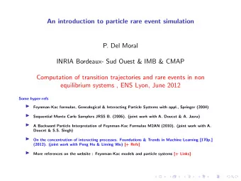
An introduction to particle simulation of rare events

• P. Del Moral

Centre INRIA de Bordeaux - Sud Ouest

Post-graduate course on ”Advanced Optimisation Techniques”, CSC Doctorate School. Luxembourg University Lecture 3

• P. Del Moral (INRIA)

INRIA Bordeaux-Sud Ouest 1 / 36

Outline

1

Introduction, motivations

2

Particle interpretations of Feynman-Kac models

3

Additive functionals

4

Normalizing constant estimation

5

Some references

• P. Del Moral (INRIA)

INRIA Bordeaux-Sud Ouest 2 / 36

Summary

1

Introduction, motivations Some rare event problems Stochastic models Importance sampling techniques The heuristic of particle methods 3 types of occupation measures

2

Particle interpretations of Feynman-Kac models

3

Additive functionals

4

Normalizing constant estimation

5

Some references

• P. Del Moral (INRIA)

INRIA Bordeaux-Sud Ouest 3 / 36

Rare event analysis

Stochastic process X ⊕ Rare event A : Proba(X ∈ A) & Law((X0, . . . , Xt) | X ∈ A) ⊃ engineering/physics/biology/economics/finance : Finance : ruin/default probabilities, financial crashes, eco. crisis,... engineering : networks overload, breakdowns, engines failures,... Physics : climate models, directed polymer conformations, particle in absorbing medium, ground states of Schroedinger models. Statistics : tail probabilities, extreme random values. Combinatorics : Complex enumeration problems. Process strategies ∈ Rare event ⇒ Control and prediction. Xt = Ft(Xt−1, Wt) → Law((W0, . . . , Wt) | X ∈ A)

• P. Del Moral (INRIA)

INRIA Bordeaux-Sud Ouest 4 / 36

Stochastic models

Only 2 Ingredients

1 Physical/biological/financial process : queuing network, portfolio, volatility process, stock market evolutions, interacting/exchange economic models ... 1 Potential function (energy type, indicator, restrictions): critical level crossing, penalties functions, constraints subsets, performance levels, long range dependence...

Objectives

Estimation of the probability of the rare event. Computing the full distributions of the path of the process evolving in the critical regime prediction ⊕ control.

• P. Del Moral (INRIA)

INRIA Bordeaux-Sud Ouest 5 / 36

Twisted Monte Carlo methods

P(X ∈ A) = 10−10 Find Q s.t. Q(A) ≃ 1 Elementary Monte Carlo estimate X i iid Q P(A) :=

• dP

dQ(x) 1A(x) Q(dx) ≃ PN(A) := 1 N

• 1≤i≤N

dP dQ(X i) 1A(X i) Variance ≃

• dP

dQ(x) 1A(x) P(dx) (ex. cross-entropy : Q ∈ {Qa, a ∈ A})

Drawbacks

Huge variance if Q badly chosen optimal choice Q(dx) ∝ 1A(x)P(dx). Need to twist the original reference process X. Stochastic evolution X = (X0, . . . , Xn) dPn dQn (X) :=

n

• k=0

pk(Xk|Xk−1) qk(Xk|Xk−1) degenerate product martingale w.r.t. n

• P. Del Moral (INRIA)

INRIA Bordeaux-Sud Ouest 6 / 36

The heuristic of particle methods

Flow of measure with increasing sampling complexity

Rare event = cascade/series of intermediate less-rare events ( ↑ energy levels, physical gateways, index level crossings). Conditional probability flow = flow of optimal twisted measures n → ηn = Law(process | series of n intermediate events) Rare event probabilities= Normalizing constants.

Particle methods

(Sampling a genealogical type default tree model ⊕ % success or default) Explorations/Local search propositions of the solution space. Branching-Selection individuals ∈ ↑ critical regimes.

• P. Del Moral (INRIA)

INRIA Bordeaux-Sud Ouest 7 / 36

5 Examples of flow of target measures

1

ηn = Loi((X0, . . . , Xn) | ∀0 ≤ p ≤ n Xp ∈ Ap)

2

ηn(dx) ∝ e−βnV (x) λ(dx) with βn ↑

3

ηn(dx) ∝ 1An(x) λ(dx) with An ↓

4

ηn = LoiK

π ((X0, . . . , Xn) | Xn = xn).

5

ηn = Loi( X hits Bn | X hits Bn before A)

5 particle heuristics :

1

Mn-local moves ⊕ individual selections ∈ An i.e. ∼ Gn = 1An

2

MCMC local moves ηn = ηnMn ⊕ individual selections ∝ Gn = e−(βn+1−βn)V

3

MCMC local moves ηn = ηnMn ⊕ individual selections ∝ Gn = 1An+1

4

M-local moves ⊕ Selection G(x1, x2) = π(dx2)K(x2,dx1)

π(dx1)M(x1,dx2)

5

Mn-local moves ⊕ Selection-branching on upper/lower levels Bn.

• P. Del Moral (INRIA)

INRIA Bordeaux-Sud Ouest 8 / 36

Interaction/branch. process ֒ → 3 types of occupation measures

(N = 3)

• = •
• = •
• = •

Current population ֒ → 1 N

N

• i=1

δξi

n←i-th individual at time n

Genealogical tree model ֒ → 1 N

N

• i=1

δ(ξi

0,n,ξi 1,n,...,ξi n,n)←i-th ancestral line

Complete genealogical tree model ֒ → 1

N

N

i=1 δ(ξi

0,ξi 1,...,ξi n)

⊕ Empirical mean potentials [success % (Gn = 1A)] ֒ → 1 N

N

• i=1

Gn(ξi

n)

• P. Del Moral (INRIA)

INRIA Bordeaux-Sud Ouest 9 / 36

Equivalent Stochastic Algorithms :

Genetic and evolutionary type algorithms. Spatial branching models. Sequential Monte Carlo methods. Population Monte Carlo models. Diffusion Monte Carlo (DMC), Quantum Monte Carlo (QMC), ... Some botanical names ∼ = application domain areas : bootsrapping, selection, pruning-enrichment, reconfiguration, cloning, go with the winner, spawning, condensation, grouping, rejuvenations, harmony searches, biomimetics, splitting, ...

• 1950 ≤ [(Meta)Heuristics] ≤ 1996 ≤ Feynman-Kac mean field particle model
• P. Del Moral (INRIA)

INRIA Bordeaux-Sud Ouest 10 / 36

Summary

1

Introduction, motivations

2

Particle interpretations of Feynman-Kac models Quelques notations Asymptotic Analysis Nonlinear Markov chains Mean field particle interpretations Some cv. results

3

Additive functionals

4

Normalizing constant estimation

5

Some references

• P. Del Moral (INRIA)

INRIA Bordeaux-Sud Ouest 11 / 36

Some notation

E measurable state space, P(E) proba. on E, B(E) bounded meas. functions (µ, f ) ∈ P(E) × B(E) − → µ(f ) =

• µ(dx) f (x)

M(x, dy) integral operator over E M(f )(x) =

• M(x, dy)f (y)

[µM](dy) =

• µ(dx)M(x, dy)

(= ⇒ [µM](f ) = µ[M(f )] ) Bayes-Boltzmann-Gibbs transformation : G : E → [0, ∞[ with µ(G) > 0 ΨG(µ)(dx) = 1 µ(G) G(x) µ(dx) E finite ⇐ ⇒ Matrix notations µ = [µ(1), . . . , µ(d)] and f = [f (1), . . . , f (d)]′

• P. Del Moral (INRIA)

INRIA Bordeaux-Sud Ouest 12 / 36

Infinite Population N ↑ ∞ ”=” Feynman-Kac measures ≃ (Gn, Mn)

ηN

n (f ) := 1

N

N

• i=1

f (ξi

n) −

→N↑∞ ηn(f ) := γn(f ) γn(1) with the un-normalized measures : γn(f ) := E  fn(Xn)

• 0≤p<n

Gp(Xp)   [Potential functions Gn] & [Xn Markov chain ∼ transitions Mn]

Feynman-Kac models ⊃ ALL of the above heuristics

Gn = 1An, e−(βn−βn−1)V , Metropolis ratio, level crossing detect.,... ⊕ (LDP)Twisted meas. : P(Vn(Xn) ≥ a) & Loi((X0, ..., Xn)|Vn(Xn) ≥ a) eλVn(Xn) P(Xn ∈ .) Gn(Xn−1, Xn) = eλ[Vn(Xn)−Vn−1(Xn−1)] Xn = (X ′

0, . . . , X ′ n) Vn(Xn) = sup 0≤p≤n

Up(X ′

p)

• P. Del Moral (INRIA)

INRIA Bordeaux-Sud Ouest 13 / 36

A first ”detailed” example

Boltzmann-Gibbs Measures : ηn(dx) = 1 Zn e−βnV (x) λ(dx) Feynman-Kac representation : ηn(f ) := γn(f ) γn(1) with γn(f ) := E  fn(Xn)

• 0≤p<n

e−(βp+1−βp)V (Xp)   and P (Xn ∈ dxn | Xn−1 = xn−1) = Mn(xn−1, dxn) with ηn = ηnMn Note : Zn = λ

• e−βnV

= λ

• e−(βn−βn−1)V e−βn−1V

λ (e−βn−1V )

• ηn−1(e−(βn−βn−1)V )

× Zn−1

(β0=0)

=

• 0≤p<n

ηp

• e−(βp+1−βp)V
• P. Del Moral (INRIA)

INRIA Bordeaux-Sud Ouest 14 / 36

A second ”detailed” example

Restriction of measures : An ↓ (Ex.: An = [an, ∞[ tails probab.) ηn(dx) = 1 Zn 1An(x) λ(dx) Feynman-Kac representation : ηn(f ) := γn(f ) γn(1) with γn(f ) := E  fn(Xn)

• 0≤p<n

1Ap+1(Xp)   and P (Xn ∈ dxn | Xn−1 = xn−1) = Mn(xn−1, dxn) with ηn = ηnMn Note : Zn = λ (An) = λ

• 1An 1An−1
• λ
• 1An−1
• ηn−1(1An )

× Zn−1

(A0=E)

=

• 0≤p<n

ηp

• 1Ap+1
• P. Del Moral (INRIA)

INRIA Bordeaux-Sud Ouest 15 / 36

Path space measures= Same math. models

Historical process : Xn := (X ′

0, . . . , X ′ n) ∈ En = (E ′ 0 × . . . × E ′ n)

⇓ Path space particles : ξi

n :=

• ξi

0,n, ξi 1,n, . . . , ξi n,n

• ∈ En = (E ′

0 × . . . × E ′ n)

⇓ ηN

n (f ) := 1

N

N

• i=1

fn(ξi

n) −

→N↑∞ ηn(fn) := γn(fn) γn(1) with the un-normalized Feynman-Kac meas. on paths spaces : γn(fn) = E  fn (X ′

0, . . . , X ′ n)

• 0≤p<n

Gp

• X ′

0, . . . , X ′ p

• 

 Example ֒ → ηn = Law((X ′

0, . . . , X ′ n) | without intersections)

X ′ = Random walk ∈ Zd & Gn (X ′

0, . . . , X ′ n) = 1{X ′

0,...,X ′ n−1}(X ′

n)

• P. Del Moral (INRIA)

INRIA Bordeaux-Sud Ouest 16 / 36

Nonlinear Markov chains

Flows of Feynman-Kac measures

ηn

Correction/mise ` a jour

− − − − − − − − − − − − − − − → ηn = ΨGn(ηn)

Pr´ ediction/exploration

− − − − − − − − − − − − − − − − − − − → ηn+1 = ηnMn+1

Nonlinear transport formulae

ΨGn(ηn) = ηnSn,ηn with Sn,ηn(x,.) := ǫnGn(x) δx + (1 − ǫnGn(x)) ΨGn(ηn) ⇓ ηn+1 = ηn (Sn,ηnMn+1) := ηnKn+1,ηn

• P. Del Moral (INRIA)

INRIA Bordeaux-Sud Ouest 17 / 36

Nonlinear Markov chains ηn = Law(X n)=Perfect sampling algorithm

Nonlinear transport formulae : ηn+1 = ηnKn+1,ηn with the collection of Markov probability transitions : Kn+1,ηn = Sn,ηnMn+1 Local transitions : P(X n ∈ dxn | X n−1) = Kn,ηn−1(X n−1, dxn) avec ηn−1 = Law(X n−1) McKean measures (canonical process) : Pn(d(x0, . . . , xn)) = η0(dx0) K1,η0(x0, dx1) . . . Kn,ηn−1(xn−1, dxn)

• P. Del Moral (INRIA)

INRIA Bordeaux-Sud Ouest 18 / 36

Mean field particle interpretations

Sampling pb ⇒ Mean field particle interpretations

Markov Chain ξn = (ξ1

n, . . . , ξN n ) ∈ E N n s.t.

ηN

n := 1

N

• 1≤i≤N

δξi

n ≃N↑∞ ηn

Approximated local transitions (∀1 ≤ i ≤ N) ξi

n−1 ξi n ∼ Kn,ηN

n−1(ξi

n−1, dxn)

• P. Del Moral (INRIA)

INRIA Bordeaux-Sud Ouest 19 / 36

Schematic picture : ξn ∈ E N

n ξn+1 ∈ E N n+1

ξ1

n Kn+1,ηN

n

− − − − − − − − − − → . . . ξi

n

− − − − − − − − − − → . . . ξN

n

− − − − − − − − − − → ξ1

n+1

. . . ξi

n+1

. . . ξN

n+1

Rationale : ηN

n

≃N↑∞ ηn = ⇒ Kn+1,ηN

n

≃N↑∞ Kn+1,ηn = ⇒ ξi ∼ i.i.d. copies of X ⇓ Particle McKean measures : 1 N

N

• i=1

δ(ξi

0,...,ξi n) −

→N↑∞ Law(X 0, . . . , X n)

• P. Del Moral (INRIA)

INRIA Bordeaux-Sud Ouest 20 / 36

Feynman-Kac models ⇔ Genetic type stochastic algo.

ξ1

n

. . . ξi

n

. . . ξN

n

       

Sn,ηN

n

− − − − − − − − − − →         

• ξ1

n Mn+1

− − − − − − − − − − → . . .

• ξi

n

− − − − − − − − − − → . . .

• ξN

n

− − − − − − − − − − → ξ1

n+1

. . . ξi

n+1

. . . ξN

n+1

        Acceptance/Rejection-Selection : [Geometric type clocks] Sn,ηN

n (ξi

n, dx)

:= ǫnGn(ξi

n) δξi

n(dx) +

• 1 − ǫnGn(ξi

n)

N

j=1 Gn(ξj

n)

PN

k=1 Gn(ξk n)δξj n(dx)

• Ex. : Gn = 1A Gn(ξi

n) = 1A(ξi n)

• P. Del Moral (INRIA)

INRIA Bordeaux-Sud Ouest 21 / 36

Some key advantages

Mean field models=stochastic linearization/perturbation technique : ηN

n = ηN n−1Kn,ηN

n−1 +

1 √ N W N

n

avec W N

n ≃ Wn Centered Gaussian Fields ⊥.

ηn = ηn−1Kn,ηn−1 stable ⇒ No propagation of local sampling errors = ⇒ Uniform control w.r.t. the time horizon ”No burning, no need to study the stability of MCMC models”. Stochastic adaptive grid approximation Nonlinear system ”positive-benefic interactions. Simple and natural sampling algorithm.

• P. Del Moral (INRIA)

INRIA Bordeaux-Sud Ouest 22 / 36

”Asymptotic” theory: TCL,PGD, PDM,...(n,N). some examples :

Empirical processes : sup

n≥0

sup

N≥1

√ N E(ηN

n − ηnp Fn) < ∞

Concentration inequalities uniform w.r.t. time : sup

n≥0

P(|ηN

n (fn) − ηn(fn)| > ǫ) ≤ c exp −(Nǫ2)/(2 σ2)

+ Guionnet supn≥0 (IHP 01) & Ledoux supFn (JTP 00) & Rio hal-09 Propagations of chaos (+Patras,Rubenthaler (AAP 09-10) : PN

n,q

:= Loi(ξ1

n, . . . , ξq n)

≃ η⊗q

n

+ 1 N ∂1Pn,q + . . . + 1 Nk ∂kPn,q + 1 Nk+1 ∂k+1PN

n,q

with supN≥1 ∂k+1PN

n,qtv < ∞ & supn≥0∂1Pn,qtv ≤ c q2.

• P. Del Moral (INRIA)

INRIA Bordeaux-Sud Ouest 23 / 36

Summary

1

Introduction, motivations

2

Particle interpretations of Feynman-Kac models

3

Additive functionals

4

Normalizing constant estimation

5

Some references

• P. Del Moral (INRIA)

INRIA Bordeaux-Sud Ouest 24 / 36

Additive functionals (with Doucet & Singh Hal-INRIA july 09)

Path space models Pn := Law(X0, . . . , Xn) dQn := 1 Zn   

• 0≤p<n

Gp(Xp)    dPn

• Hyp. : Mn(xn−1, dxn) = Hn(xn−1, xn) λn(dxn)

⇒ Qn(d(x0, . . . , xn)) = ηn(dxn) Mn,ηn−1(xn, dxn−1) . . . M1,η0(x1, dx0) with the backward transitions : Mp+1,η(x, dx′) ∝ Gp(x′) Hp+1(x′, x) η(dx′) Particle estimates ∼ complete genealogical tree : QN

n (d(x0, . . . , xn)) = ηN n (dxn) Mn,ηN

n−1(xn, dxn−1) . . . M1,ηN 0 (x1, dx0)

• P. Del Moral (INRIA)

INRIA Bordeaux-Sud Ouest 25 / 36

2 type of path-space estimates

Complete genealogical tree = ⇒ McKean meas. ⊕ FK-Path space 1 N

N

• i=1

δ(ξi

0,...,ξi n) ≃N Loi(X 0, . . . , X n)

& QN

n ≃N Qn

Simple genealogical tree = ⇒ FK-Path space ηN

n = 1

N

N

• i=1

δ(ξi

0,n,ξi 1,n,...,ξi n,n) ≃N Qn = ηn

• P. Del Moral (INRIA)

INRIA Bordeaux-Sud Ouest 26 / 36

Some estimates

Additive functional (with Doucet & Singh Hal-INRIA july 09) : Fn(x0, . . . , xn) = 1 n + 1

• 0≤p≤n

fp(xp) Bias estimate+uniform Lp-bounds + variance N E

• [(QN

n − Qn)(Fn)]2

≤ c × (1/n + 1/N) Uniform exponential concentration 1 N log sup

n≥0

P

• [QN

n − Qn](Fn)

• ≥

b √ N + ǫ

• ≤ −ǫ2/(2b2)
• P. Del Moral (INRIA)

INRIA Bordeaux-Sud Ouest 27 / 36

Summary

1

Introduction, motivations

2

Particle interpretations of Feynman-Kac models

3

Additive functionals

4

Normalizing constant estimation A key multiplicative formula Some examples Convergence analysis

5

Some references

• P. Del Moral (INRIA)

INRIA Bordeaux-Sud Ouest 28 / 36

Problem : Un-normalized measures estimation

γn(f ) := E  fn(Xn)

• 0≤p<n

Gp(Xp)   ≃N↑∞ γN

n (f ) := ???

Key observation : ηn(Gn) γn(1) = γn(Gn) = γn+1(1)

= ⇒ Multiplicative formula unbias particle estimates

γn(1) =

• 0≤p<n

ηp(Gp) ← −N↑∞ γN

n (1) :=

• 0≤p<n

ηN

p (Gp)

⇓ γn(f ) := γn(1) × ηn(f ) ← −N↑∞ γN

n (f ) := γN n (1) × ηN n (f )

• Note. : If Gn takes null values (ex. Gn = 1A) ⇒ convention = we estimate by 0.
• P. Del Moral (INRIA)

INRIA Bordeaux-Sud Ouest 29 / 36

2 Examples : Feynman-Kac models

Tube confinement : γn(1)

Gn=1A

= P (∩0≤p<nXp ∈ A) ≃N↑∞ γN

n (1) :=

• 0≤p<n

ηN

p (A)

Self avoiding walks : γn+1(1) = P (∀p < q ≤ n Xp = Xq) = 1 (2d)n Card {s.a.w. with length =n} ≃N↑∞ γN

n+1(1) :=

• 0≤p≤n

empirical mean potential at time p Several strategies :

1

Path evolutions with G-intersection detection

2

Local transitions without intersections with G-future proba. of intersection.

3

...

• P. Del Moral (INRIA)

INRIA Bordeaux-Sud Ouest 30 / 36

+2 Examples : Boltzmann-Gibbs static measures

Partition functions:

• Gn = e−(βn+1−βn)V

et (ηnMn = ηn) ⇒ dηn ∝ e−βnV dλ

• Note :

λ

• e−βnV

= λ

• Gn × e−βn−1V

= ηn (Gn) λ

• e−βn−1V

⇓ λ

• e−βnV

= γn(1) ≃N↑∞ γN

n (1) :=

• 0≤p<n

ηN

p

• e−(βp+1−βp)V

Volumes and Cardinals : (Gn = 1An+1) and (ηnMn = ηn) = ⇒ ηn(dx) ∝ 1An+1 λ(dx) ⇓ λ (An) = γn(1) ≃N↑∞ γN

n (1) :=

• 0≤p≤n

ηN

p (Ap+1)

• P. Del Moral (INRIA)

INRIA Bordeaux-Sud Ouest 31 / 36

Convergence analysis

Asymptotic theory : fluctuations & deviations + A. Guionnet (AAP 99, SPA 98), + L. Miclo (SP 2000), + D. Dawson Non asymptotic theory : bias and variance estimates

1

Taylor type expansion (+Patras & Rubenthaler (AAP 09) : E

• (γN

n )⊗q(F)

• =: QN

n,q(F) = γ⊗q n (F) +

• 1≤k≤(q−1)(n+1)

1 Nk ∂kQn,q(F) [Hyp.∼ simple genetic algo. ǫn = 0 & potentiel > 0]

2

Variance estimates (+Cerou & Guyader Hal-INRIA nov.08) : E

• γN

n (fn) − γn(fn)

2 ≤ c n N × γn(1)2

• Hyp. + weak conditions ⊃ :

Mean field models with acceptance rate ∀ǫn ≥ 0. Potential functions ≥ 0 (⊃ indicator functions). Path space models Xn = (X ′

0, . . . , X ′ n), with X ′ ” mixing”.

• P. Del Moral (INRIA)

INRIA Bordeaux-Sud Ouest 32 / 36

Summary

1

Introduction, motivations

2

Particle interpretations of Feynman-Kac models

3

Additive functionals

4

Normalizing constant estimation

5

Some references

• P. Del Moral (INRIA)

INRIA Bordeaux-Sud Ouest 33 / 36

some references + http links

Particle methods & Sequential Monte Carlo

Feynman-Kac formulae. Genealogical and interacting particle systems, Springer (2004) ⊕ Refs. (with L. Miclo) Branching and Interacting Particle Systems Approximations of Feynman-Kac Formulae. S´ eminaire de Probabilit´ es XXXIV, Lecture Notes in Mathematics, Springer-Verlag Berlin, Vol. 1729, 1-145 (2000). (with Doucet A. et Jasra A.) Sequential Monte Carlo Samplers. JRSS B (2006). (with A. Doucet) On a class of genealogical and interacting Metropolis models. S´

• em. de Proba. 37 (2003).

(with F. Patras et S. Rubenthaler) Coalescent tree based functional representations for some Feynman-Kac particle models, to appear in : Annals of Applied Probability (2009)

• P. Del Moral (INRIA)

INRIA Bordeaux-Sud Ouest 34 / 36

Rare event analysis

Particle simulation of twisted measures (with J. Garnier) Genealogical Particle Analysis of Rare

• events. Annals of Applied Probab., 15-4 (2005).

(with J. Garnier) Simulations of rare events in fiber optics by interacting particle systems. Optics Communications, Vol. 267 (2006). Branching processes (with P. Lezaud) Branching and interacting particle interpretation of rare event proba.. Stochastic Hybrid Systems : Theory and Safety Critical Applications, eds. H. Blom and J.

• Lygeros. Springer (2006).

(with F. Cerou, Le Gland F., Lezaud P.) Genealogical Models in Entrance Times Rare Event Analysis, Alea, Vol. I, (2006). Proceedings Conf. RESIM 2006 (with A. M. Johansen et A. Doucet) Sequential Monte Carlo Samplers for Rare Events (with F. Cerou, A. Guyader, F. LeGland, P. Lezaud et H. Topart) Some recent improvements to importance splitting

• P. Del Moral (INRIA)

INRIA Bordeaux-Sud Ouest 35 / 36

Absorption models

(with L. Miclo) Particle Approximations of Lyapunov Exponents Connected to Schrodinger Operators and Feynman-Kac

• Semigroups. ESAIM Probability & Statistics, vol. 7, pp. 169-207 (2003).

(avec A. Doucet) Particle Motions in Absorbing Medium with Hard and Soft Obstacles. Stochastic Analysis and Applications, vol. 22 (2004).

+ recent preprints

(with A. Doucet and S. S. Singh) A Backward Particle Interpretation of Feynman-Kac Formulae (HAL-INRIA 2009) (with A. Doucet and S. S. Singh) Forward Smoothing Using Sequential Monte Carlo Technical Report 638. Cambridge University Engineering Department (2009). (with F. Cerou et A. Guyader) A non asymptotic variance theorem for unnormalized Feynman-Kac particle models (HAL-INRIA 2008). (avec A. Doucet et A. Jasra) On Adaptive Resampling Procedures for Sequential Monte Carlo Methods (HAL-INRIA 2008).

• P. Del Moral (INRIA)

INRIA Bordeaux-Sud Ouest 36 / 36