AN INTRODUCTION TO NEURAL NETWORKS Scott Kuindersma November 12, - PowerPoint PPT Presentation
AN INTRODUCTION TO NEURAL NETWORKS Scott Kuindersma November 12, 2009 SUPERVISED LEARNING We are given some training data: We must learn a function If y is discrete, we call it classification If it is continuous, we call it
AN INTRODUCTION TO NEURAL NETWORKS Scott Kuindersma November 12, 2009
SUPERVISED LEARNING • We are given some training data: • We must learn a function • If y is discrete, we call it classification • If it is continuous, we call it regression
ARTIFICIAL NEURAL NETWORKS • Artificial neural networks are one technique that can be used to solve supervised learning problems • Very loosely inspired by biological neural networks • real neural networks are much more complicated, e.g. using spike timing to encode information • Neural networks consist of layers of interconnected units
PERCEPTRON UNIT • The simplest computational neural unit is called a perceptron • The input of a perceptron is a real vector x • The output is either 1 or -1 • Therefore, a perceptron can be applied to binary classification problems • Whether or not it will be useful depends on the problem... more on this later...
PERCEPTRON UNIT [MITCHELL 1997]
SIGN FUNCTION
EXAMPLE • Suppose we have a perceptron with 3 weights: • On input x 1 = 0.5, x 2 = 0.0 , the perceptron outputs: • where x 0 = 1
LEARNING RULE • Now that we know how to calculate the output of a perceptron, we would like to find a way to modify the weights to produce output that matches the training data • This is accomplished via the perceptron learning rule • for an input pair where, again, x 0 = 1 • Loop through the training data until (nearly) all examples are classified correctly
MATLAB EXAMPLE
LIMITATIONS OF THE PERCEPTRON MODEL • Can only distinguish between linearly separable classes of inputs • Consider the following data:
PERCEPTRONS AND BOOLEAN FUNCTIONS • Suppose we let the values (1,-1) correspond to true and false , respectively • Can we describe a perceptron capable of computing the AND function? What about OR ? NAND ? NOR ? XOR ? • Let’s think about it geometrically
BOOLEAN FUNCS CONT’D AND OR NAND NOR
EXAMPLE: AND • Let p AND (x1,x2) be the output of the perceptron with weights w 0 = -0.3, w 1 = 0.5, w 2 = 0.5 on input x 1 , x 2 x 1 x 2 p AND (x1,x2) -1 -1 -1 -1 1 -1 1 -1 -1 1 1 1
XOR
XOR • XOR cannot be represented by a perceptron, but it can be represented by a small network of perceptrons, e.g., x 1 OR x 2 AND x 1 NAND x 2
PERCEPTRON CONVERGENCE • The perceptron learning rule is not guaranteed to converge if the data is not linearly separable • We can remedy this situation by considering linear unit and applying gradient descent • The linear unit is equivalent to a perceptron without the sign function. That is, its output is given by: • where x 0 = 1
LEARNING RULE DERIVATION • Goal: a weight update rule of the form • First we define a suitable measure of error • Typically we choose a quadratic function so we have a global minimum
ERROR SURFACE [MITCHELL 1997]
LEARNING RULE DERIVATION • The learning algorithm should update each weight in the direction that minimizes the error according to our error function • That is, the weight change should look something like
GRADIENT DESCENT
GRADIENT DESCENT • Good: guaranteed to converge to the minimum error weight vector regardless of whether the training data are linearly separable (given that α is sufficiently small) • Bad: still can only correctly classify linearly separable data
NETWORKS • In general, many-layered networks of threshold units are capable of representing a rich variety of nonlinear decision surfaces • However, to use our gradient descent approach on multi-layered networks, we must avoid the non-differentiable sign function • Multiple layers of linear units can still only represent linear functions • Introducing the sigmoid function ...
SIGMOID FUNCTION
SIGMOID UNIT [MITCHELL 1997]
EXAMPLE • Suppose we have a sigmoid unit k with 3 weights: • On input x 1 = 0.5, x 2 = 0.0 , the unit outputs:
NETWORK OF SIGMOID UNITS o 2 o 4 o 3 2 3 4 output layer w 02 0 1 hidden layer w 31 x 0 x 1 x 2 x 3
EXAMPLE 3 1.0 .5 -.5 1 2 .1 .2 3.2 .3 0 -.2 x 0 x 1 x 2
EXAMPLE 3 0.8 1.0 .5 -.5 0.75 1 2 output 0.7 2 0.65 .1 1 .2 3.2 .3 0 0 -.2 2 1.5 1 − 1 0.5 0 x 0 − 0.5 − 1 x 1 x 2 − 1.5 − 2 x1 − 2 x2
BACK-PROPAGATION • Really just applying the same gradient descent approach to our network of sigmoid units • We use the error function:
BACKPROP ALGORITHM
BACKPROP CONVERGENCE • Unfortunately, there may exist many local minima in the error function • Therefore we cannot guarantee convergence to an optimal solution as in the single linear unit case • Time to convergence is also a concern • Nevertheless, backprop does reasonably well in many cases
MATLAB EXAMPLE • Quadratic decision boundary • Single linear unit vs. Three-sigmoid unit backprop network... GO!
BACK TO ALVINN • ALVINN was a 1989 project at CMU in which an autonomous vehicle learned to drive by watching a person drive • ALVINN's architecture consists of a single hidden layer back- propagation network • The input layer of the network is a 30x32 unit two dimensional "retina" which receives input from the vehicles video camera • The output layer is a linear representation of the direction the vehicle should travel in order to keep the vehicle on the road
ALVINN
REPRESENTATIONAL POWER OF NEURAL NETWORKS • Every boolean function can be represented by a network with two layers of units • Every bounded continuous function can be approximated to arbitrarily accuracy by a two-layer network of sigmoid hidden units and linear output units • Any function can be approximated to arbitrarily accuracy by a three layer network sigmoid hidden units and linear output units
READING SUGGESTIONS • Mitchell, Machine Learning , Chapter 4 • Russell and Norvig, AI a Modern Approach , Chapter 20
Recommend
More recommend
Explore More Topics
Stay informed with curated content and fresh updates.
