An Equilibrium Theory of Learning, Search and Wages Francisco - - PowerPoint PPT Presentation

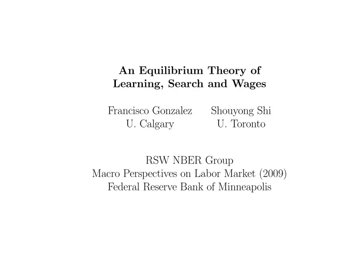
An Equilibrium Theory of Learning, Search and Wages Francisco Gonzalez Shouyong Shi

• U. Calgary
• U. Toronto

RSW NBER Group Macro Perspectives on Labor Market (2009) Federal Reserve Bank of Minneapolis

• 1. Tasks and Motivation
• Formulate the problem of learning

by unemployed workers about themselves

• characterize equilibrium with such learning
• examine how reemployment wages and rates

depend on search history

2

What’s the story?

• workers do not know their ability/productivity

— some are lucky to find jobs = ⇒ revise beliefs upward — some are not so lucky = ⇒ discouragement

• divergence in histories =

⇒ endogenous heterogeneity in: — workers’ beliefs about their job-finding process — search decisions — job-finding rates and wages

3

Specific facts:

• average job-finding prob decreases with duration
• wage losses increase with unemployment duration:

— US Displaced Worker Survey (Addison and Portugal 89): increasing duration by 100% reduces wages by 10% — UK Labour Force Survey (Gregg and Wadsworth 00): duration of 7-12 months = ⇒ wage loss of 27 log points

4

Other complementary theories:

• unobserved worker heterogeneity,

and long duration is a signal of low productivity

• skill depreciation during unemployment
• declining wealth/benefit during unemployment

5

Why use an equilibrium?

• need to explain the above facts as market outcomes
• firms can adjust offers and vacancies to respond to learning:

— with exogenous wages, low-wage jobs would be filled more quickly as reservation wages fall

6

• 2. Model Environment

Workers and jobs:

• firms or jobs: free entry
• workers (risk neutral):

— unemployed workers search — employed workers produce y > 0, shock of separation into unemployment: δ — shock of exit from market: σ

7

Worker’s unknown ability:

• new worker draws ability i ∈ {H, L}:

— unknown, permanent, prob(H) = p

• worker’s productivity is a random variable:

½ y > 0, prob ai 0, prob 1 − ai — H is more “productive”: 0 < aL < aH < 1 — realized immediately after contact

8

Directed search:

• continuum of submarkets x ∈ X = [0, 1/aH]

x: prob of getting productive match (per search unit); W (x): wage level; λ (x): tightness

• search choice:

a submarket x to enter (tradeoff between x and W)

9

Matching in submarket x:

• total number of (productive) matches: F(ue (x) , v (x))
• total productive units of search in submarket x:

ue (x) = aH × uH (x) + aL × uL (x) ui (x): # of type-i workers in submarket x

10

Matching in submarket x (continued):

• matching probability per productive (search) unit:

x = F(ue(x), v(x))

ue(x)

= F(1, v(x) ue(x) | {z } ) tightness λ(x)

• matching probabilities for participants:

type-H type-L vacancy aH x aL x

F v = x λ(x)

11

Wage function W(x):

• free-entry of vacancies:

Jv (x) ≤ 0 and v (x) ≥ 0 for all x ∈ X with complementary slackness

12

• firm’s expected profit of vacancy in market x:

Jv(x) = −c + x λ(x) × (1 − σ) × Jf(W(x))

• firm’s value of employing worker at w,

discounted to the end of previous period: Jf(w) = 1 1 + r £ y − w + (1 − σ) × (1 − δ) × Jf(w) ¤

13

Wage function W(x):

• free entry implies wage function:

W(x) = y − cA λ(x) x , A ≡ δ + r + σ 1 − σ

• W 0(x) < 0 (tradeoff between W and matching prob x)

14

• 3. Learning in directed search equilibrium

Information and learning:

• match success and failure contain info about ai

— info content depends on x: aLx < aHx

• firms do not face signal extraction:

matching prob x/λ(x) and wage W(x) are known

• all participants know all statistics in all submarkets

15

Worker’s beliefs: expected value of his a

• common initial belief: μ0 = p aH + (1 − p) aL
• belief before search in a period: μ = PH aH + PL aL
• posterior prob after search outcome:

P(ai | x, success) = ai x

μ xPi = ai μPi

P(ai | x, failure) = 1−xai

1−xμPi

16

Updating beliefs:

• beliefs before and after search:

μ → ⎧ ⎪ ⎨ ⎪ ⎩ E (a | x, success) = aH + aL − aHaL/μ ≡ φ(μ) E(a | x, failure) = aH − 1−xaL

1−xμ (aH − μ) ≡ H(x, μ)

• properties of updating:

— beliefs obey a Markov process — μ is sufficient statistic for search history — search in market with higher x is more informative

17

Rule out experimentation (sufficient condition): y − b c > [A + aHx∗] λ0(x∗) − aHλ(x∗) x∗ is defined by: λ0(x∗) = aHλ( 1 aH )

18

Search decision of a worker with belief μ:

• value of being employed at wage w,

discounted to the end of previous period: Je(μ, w) = 1 1 + r {w + (1 − σ) [(1 − δ) Je(μ, w) + δ V (μ)]}

• return to search in market x:

R(x, μ) ≡ xμ Je(φ(μ), W(x)) + (1 − xμ) V (H(x, μ))

19

Search decision of a worker with belief μ (continued):

• search decision:

(1 + r) V (μ) = b + (1 − σ) × max

x∈X R(x, μ)

• policy functions:

— search choice (of submarket): x = g(μ) ∈ G(μ) — desired wage: w(μ) = W(g(μ))

20

Stationary symmetric equilibrium:

• Block 1: individual decisions and market tightness

(i) given W (.), workers with belief μ choose x = g(μ) ∈ G (μ) (ii) workers update beliefs according to φ(μ) and H(g(μ), μ) (iii) W(.) satisfies free-entry condition (iv) consistency: λ (x) = v(x)

ue(x) for all x with v (x) > 0

• Block 2:

(v) distribution of workers consistent with law of motion Equilibrium is block recursive (as in Shi 09)

21

• 4. Monotonicity of desired wages

Want to show:

• policy function, w (μ) = W (g (μ)), is strictly increasing

— i.e., wages fall as beliefs deteriorate — i.e., search decision x = g (μ) strictly decreases in μ Problems:

• value V (μ) is convex;
• V 0(μ) may not exist; FOC may not be applicable

22

A map of our approach:

• use lattice-theoretic methods to prove:

policy function is monotone

• monotone policy function + convex value function

= ⇒ validate first-order condition

• the above results + first principles of calculus

= ⇒ envelope condition + differentiability of V

23

Topkis’ Theorems (98): max

z∈−X f(z, μ),

z = −x; μ ∈ M

• If f is supermodular in (z, μ),

(and if (−X) × M is a lattice), then max Z (μ) and min Z (μ) are increasing in μ

• If f is strictly supermodular in (z, μ),

then every selection z (μ) ∈ Z (μ) is increasing in μ.

24

Use lattice-theoretic techniques:

• transform payoff function:

ˆ R(z, μ) ≡ R(x, μ) μ , z ≡ −x

• optimal search decision z(μ) ∈ Z(μ):

(1 + r) V (μ) = b + (1 − σ) × μ × max

z∈−X

ˆ R (z, μ)

25

Theorem 4.1: monotonicity of desired wages Assume separation rate satisfies 0 ≤ δ ≤ ¯ δ. Then

• ˆ

R(z, μ) is strictly supermodular in (z, μ)

• every selection z(μ) ∈ Z(μ) is an increasing function;

every selection x = g(μ) is a decreasing function

• w(μ) = W (g (μ)) is an increasing function

26

Why is ˆ R(z, μ) strictly supermodular? μ ⎧ ⎪ ⎪ ⎪ ⎨ ⎪ ⎪ ⎪ ⎩ expected value:

• prob. xμ

− − − − − − − − − → φ(μ); δ × xμφ(μ) + μxW(x)

• prob. (1 − xμ)

− − − − − − − − − − → H(x, μ); m ≡ (1 − xμ)H(x, μ) High x submarkets have low wages:

• failure in higher x =

⇒ deeper discouragement: ∂m

∂x < 0

• marginal “damage” of x increases in μ:

∂ ∂μ

h

∂m ∂x

i < 0

27

Why is ˆ R(z, μ) strictly supermodular? (cont’d)

• convexity of V is important:

properties above carry over to payoff only for convex V : ˆ R = −z W(−z) A(1 − σ) − δ A z V (φ(μ)) | {z } + (1 μ + z) V (H(z, μ)) | {z } expected payoff to success to failure

• assumption δ ≤ ¯

δ is needed

28

Theorem 4.1 (continued): strict monotonicity Assume 0 < δ ≤ ¯ δ. Statements below are equivalent:

• (i) V (μ) is strictly convex for all μ
• (ii) every selection z(μ) ∈ Z(μ) is strictly increasing
• (iii) corner z = −1/aH is not optimal for any μ > aL
• (iv) corner z = −1/aH is not optimal for μ = aH
• (v) y−b

c

< (A + 1)λ0( 1

aH) − aHλ( 1 aH)

29

Why linear V over some beliefs = ⇒ even most optimistic workers search for lowest wage?

• V (μ) being linear in [μa, μb]

= ⇒ decision problem is strictly concave for such μ = ⇒ optimal choice of z is unique for such μ

• strict supermodularity of ˆ

R = ⇒ monotonicity of optimal decisions = ⇒ unique maximizer is corner, {−1/aH}, for such μ

30

Why linear V over some beliefs = ⇒ even most optimistic workers search for lowest wage?

• V (μ) linear in [μa, μb] =

⇒ unique maximizer is {−1/aH}

• Same argument applies to μ ∈

£ φi(μa), φi(μb) ¤ , i ≥ 1: unique maximizer is {−1/aH} for all such μ

• limi→∞ φi(μ) → aH,

and Z(μ) is upper hemicontinuous = ⇒ {−1/aH} ∈ Z(aH).

31

• 5. Uniqueness and differentiability

Theorem 5.1:

• optimal choices obey first-order condition
• generalized envelope theorem holds
• from the point where a worker has a match failure,

— value function is differentiable — optimal choice is unique

32

Why is V differentiable at a match failure?

• Suppose V not differentiable at μτ+1 = H(z(μτ), μτ)

= ⇒ multiple choices will be optimal in (τ + 1), = ⇒ V 0(μ−

τ+1) < V 0 ¡

μ+

τ+1

¢

• worker can gain by raising z slightly above z (μτ)

(i.e., searching in submarket with slightly higher w) — next period beliefs slightly above μτ+1 — marginal benefit increases by a discrete amount — matching prob decreases continuously

33

• 5. Implications
• unemployment duration =

⇒ wage losses, discouragement

• wage dispersion among identical workers
• what about average job-finding prob in a cohort?

— searching for easier jobs increases job-finding — but average ability in a cohort deteriorates with duration

34

Implications (continued):

• reemployment and wages depend on entire history:

past occurrences of unemployment, past spells, etc.

• history can be summarized by beliefs entering unemployment

and, hence, by worker’s pre-unemployment wage

• even without skill differences, higher pre-unemp wage

— increases reemployment wages; — may induce longer duration

35

• 6. Conclusion
• tractable equilibrium theory of learning:

block recursivity; lattice-theoretic in dynamic prog

• discouragement during search:

longer search = ⇒ more pessimistic = ⇒ wage losses

• endogenous heterogeneity useful for:

understanding wage formation, duration dependence, etc.

• learning + aggregate fluctuations?

36