An Efficient Gauss-Newton Algorithm for Symmetric Low-Rank Product - PowerPoint PPT Presentation
An Efficient Gauss-Newton Algorithm for Symmetric Low-Rank Product Matrix Approximations Xin Liu State Key Laboratory of Scientific and Engineering Computing Institute of Computational Mathematics and Scientific/Engineering Computing Academy of
An Efficient Gauss-Newton Algorithm for Symmetric Low-Rank Product Matrix Approximations Xin Liu State Key Laboratory of Scientific and Engineering Computing Institute of Computational Mathematics and Scientific/Engineering Computing Academy of Mathematics and Systems Science Chinese Academy of Sciences, China (Joint work with Zaiwen Wen 1 , Yin Zhang 2 ) 2014 Workshop on Optimization for Modern Computation, BICMR, Peking University September 3, 2014 1 Peking University, China 2 Rice University, U.S. Xin Liu (AMSS) SLRPGN September 3, 2014 1 / 29
Original Motivation Low-rank approximation : given B ∈ R n × m and k < min ( n , m ) , � XZ T − B � F : X ∈ R n × k , Z ∈ R m × k � � min X , Z Closely related to SVD k -Dominant ( k -D) SVD of n × m ⇒ solution Solution + QR( n × k ) and SVD ( k × k ) ⇒ k -D SVD of n × m How about the symmetric case? for A = A T ∈ R n × n (e.g., A = BB T ), � XX T − A � F : X ∈ R n × k � � min X Xin Liu (AMSS) SLRPGN September 3, 2014 2 / 29
Symmetric Low-Rank Product Optimization A nonlinear, nonconvex least squares problem X ∈ R n × k � XX T − A � 2 min F Fundamental in low-rank matrix approximations Principal subspace of A : span ( X ∗ ) = span { q 1 , q 2 , . . . , q k } where X ∗ is a global minimizer, and { q j } k j = 1 are k dominant eigenvectors of A . For A = BB T , columns of X are “principal components” of B . Xin Liu (AMSS) SLRPGN September 3, 2014 3 / 29
Most Established Eigensolvers Why not just call eigs (or svds ) in M atlab ? (ARPACK) Why not use one of the existing eigensolvers? Emerging applications demand new capacities. high efficiency at moderate accuracy high eigenspace dimensions high parallel scalability warm-start capacity Established eigensolvers often lack in one or more aspects. Advanced scientific computing and evolving computer archtectures call for new algorithms (either of general or special purpose). Xin Liu (AMSS) SLRPGN September 3, 2014 4 / 29
Block Methods Block vs. Sequential (Lanczos-type Methods) Block SpMV: AV = [ Av 1 Av 2 · · · Av k ] Sequential SpMv’s: Av → A 2 v · · · → A k v (+ inner products for orthogonalization) As k increases, block methods are gaining advantages. Block methods can be warm-started in an iterative setting. Classic Block Method SSI: (power method) X i + 1 = orth ( AX i ) Other block algorithms: Block Jacobian-Davidson: Feast Trace minimization: LOBPCG, LMSVD Research on block methods seems still largely unsettled. Xin Liu (AMSS) SLRPGN September 3, 2014 5 / 29
Trace Minimization Trace Minimization X ∈ R n × k tr ( X T AX ) X T X = I . max s.t. L.-Wen-Zhang, L imited M emory Block Krylov Subspace Optimization for Computing Dominant S ingular V alue D ecompositions, SIAM Journal on Scientific Computing , 35-3(2013); A := BB T , main iteration of LMSVD: X ( i + 1 ) = orth ( AY ( i ) ) , where Y ( i ) = argmax { φ ( X ) | X T X = I , X ∈ S k } , S k = span { X k , X k − 1 , ..., X k − p } ; LMSVD code is available at MathWorks (Google: LMSVD). Xin Liu (AMSS) SLRPGN September 3, 2014 6 / 29
Bottleneck Two main types of operations: AX & RR / orth As k increases, AX ≪ RR / orth −→ bottleneck Parallel Scalability AX −→ Ax 1 ∪ Ax 2 ∪ ... ∪ Ax k . Higher. RR / orth inherits sequentiality. Lower. Avoid bottleneck? Do less RR/orth No free lunch? Do more BLAS3 (higher scalability than AX ) Xin Liu (AMSS) SLRPGN September 3, 2014 7 / 29
Orthogonal Free Models Unconstrained Model: min X ∈ R n × k 1 4 || X T X || 2 F + 1 2 tr ( X T AX ) , Dai-Jiang-Cui, 2013 Trace-penalty Minimization X ∈ R n × k f ( X ) := 1 2 tr ( X T AX ) + µ 4 � X T X − I � 2 min F . EIGPEN, Wen-Yang-L.-Zhang, 2013, available at ”optimization online” Good properties: Equivalence to Trace Minimization does NOT require µ → ∞ No non-global local minimizer, less undesired saddle point RR/Orth mostly replaced by “big” BLAS3 Efficient for moderate accuracy, numerically stable Parallel scalability appears promising Algorithm Gradient method with Barzilai Borwein stepsize Rayleigh-Ritz restart Xin Liu (AMSS) SLRPGN September 3, 2014 8 / 29
Why New Approach? Questions to EIGPEN Gradient method + BB (How about high-order methods?) Condition number: k = 1: κ ( ∇ 2 f µ (ˆ X )) = λ n − λ 1 λ 2 − λ 1 ; k > 1: κ ( ∇ 2 f µ (ˆ X )) = 0, (How about linear convergence rate?) � tr ( S T ∇ 2 f µ (ˆ � X )( S )) : tr ( S T S ) = 1 , S T Q k = 0 max S ∈ R n × k � ∇ 2 f µ (ˆ � � X ) � κ � � Q ⊥ � tr ( S T ∇ 2 f µ (ˆ � k X )( S )) : tr ( S T S ) = 1 , S T Q k = 0 min S ∈ R n × k λ n − λ 1 = ( Explain why RR restart is useful. ) . λ k + 1 − λ k µ should be tuned in properly. (How to avoid µ ?) Solution min X ∈ R n × k � XX T − A � 2 SLRP: F Xin Liu (AMSS) SLRPGN September 3, 2014 9 / 29
Notation Let eigenvalues of A be in a descending order λ 1 ≥ λ 2 ≥ · · · ≥ λ n Eigenvalue decomposition: A = Q n Λ n Q T Q T n Q n = I , Λ n diagonal n , k -D principal eigenspace: span ( Q k ) � span { q 1 , q 2 , . . . , q k } k -D principal eigenpair: ( Q k , Λ k ) Xin Liu (AMSS) SLRPGN September 3, 2014 10 / 29
Optimal Solutions of SLRP Equivalence Assume that A = A T ∈ R n × n such that λ k ≥ 0. Then X ∈ R n × k is a solution to min � XX T − A � 2 F if and only if it has SVD: 1 k V T , X = Q k Λ 2 where ( Q k , Λ k ) is a k -D principal eigenpair of A , V ∈ R k × k is orthogonal but otherwise arbitrary. 1st-order condition for SLRP: AX = X ( X T X ) Stationary points span invariant subspaces. Xin Liu (AMSS) SLRPGN September 3, 2014 11 / 29
Gauss-Newton Review Nonlinear Least Squares Model: x ∈ R n f ( x ) � 1 r ( x ) : R n → R m . 2 r ( x ) T r ( x ) . min Linearize: r ( x + s ) ≈ r ( x ) + J ( x ) s , where J ( x ) is the Jacobian. Normal equations + Line Search: (minimize the lienar approximation) J ( x ) T J ( x ) s = − J ( x ) T r ( x ) . x = x + α s . Some properties: Fast for small residual. Slow for large residual. Local convergence may require α < 1 all the time. Xin Liu (AMSS) SLRPGN September 3, 2014 12 / 29
SLRP SLRP: Nonlinear Least Squares Model X ∈ R n × k f ( X ) � 1 R ( X ) � XX T − A . 2 � R ( X ) � 2 min F . Let J ( X ) : R n × k → R n × n be the Jacobian operator of R ( X ) at X . Normal equations: (size nk × nk ) J ( X ) T J ( X )( S ) = − J ( X ) T ( R ( X )) . Infinitely many solutions since J ( X ) is rank deficient. Xin Liu (AMSS) SLRPGN September 3, 2014 13 / 29
GN Directions Special structure of normal equations allows low-cost solution: SX T X + XS T X = AX − X ( X T X ) GN Direction Let X ∈ R n × k be full rank, and P X = X ( X T X ) − 1 X T . Then � � � I − 1 AX ( X T X ) − 1 − X � S C = 2 P X + XC , where C T = − C , satisfies the normal equations. In particular, for C = 0, � � � I − 1 AX ( X T X ) − 1 − X � S 0 = 2 P X is a minimum weighted-norm Gauss-Newton direction at X . Xin Liu (AMSS) SLRPGN September 3, 2014 14 / 29
SLRPGN (Theoretical Version) Gauss-Newton (GN): While not “converged”, do If σ min ( X ) < δ , set X = X + P ; —- Correction Step 1 � � 1 , σ 3 Select α = min min ( X ) / �∇ f ( X ) � F , set X = X + α S 0 . 2 Calculation GN step: Y = X ( X T X ) − 1 , G = AY − X S 0 = G − X ( Y T G ) / 2 Computational cost: 1 block SpMV: AY 3 dense matrix multiplications 1 k × k linear system with n rhs Xin Liu (AMSS) SLRPGN September 3, 2014 15 / 29
SLRPGN (Practical Implementation) So far, in practice α = 1 appears always to work well; Correction step can hardly be invoked. [ X , Y ] = GN ( A , X ) While not “converged”, do Y = X ( X T X ) − 1 1 X = AY − X ( Y T AY − I ) / 2 2 Simple Algorithm Two-liner with no parameters No orthogonalization No Rayleigh-Ritz (unless eigenpairs are required) Xin Liu (AMSS) SLRPGN September 3, 2014 16 / 29
Step Size and Correction Step Full Rankness: σ min ( X i + 1 ) ≥ 0 . 75 σ min ( X i ) Correction Step: � � � λ n /λ 1 λ n δ ≤ √ k 4 + 20 � λ n p UV T p , where U T X = 0 and U T U = I ) X c = X + P ( := Key properties: σ min ( X c ) ≥ δ f ( X c ) < f ( X ) − 1 4 λ 2 n Xin Liu (AMSS) SLRPGN September 3, 2014 17 / 29
Convergence Results Theorem (Global Convergence) Suppose that A ≻ 0 . Let { X i } be generated by SLRPGN(TH) starting from a full-rank initial point. Then after finite number of iterations, step-size α = 1 will always be taken, no more correction step, and ∇ f ( X i ) → 0 . f ( X ) does not have any local (non-global) minimum. It is unlikely that the iterates get trapped at a saddle point. Better local convergence result holds if we further assume λ k > λ k + 1 . Theorem (Q-Linear Rate) Suppose A ≻ 0 and λ k > λ k + 1 . Then { X i } , a sequence generated by SLRPGN(PR) starting from a full-rank initial point X 0 ∈ L ( γ ) , globally converges to L ( f ∗ ) , where L ( γ ) := { X | f ( X ) ≤ γ } denotes the level set, f ∗ denotes the global minimum of SLRP and γ > f ∗ is a constant. Moreover, the gradient sequence {∇ f ( X i ) } converges to zero at a Q-linear rate λ k + 1 λ k . Xin Liu (AMSS) SLRPGN September 3, 2014 18 / 29
Recommend
More recommend
Explore More Topics
Stay informed with curated content and fresh updates.


