UQ, STAT2201, 2017, Lecture 8 (and part of 9). Unit 8 Two Sample - PowerPoint PPT Presentation
UQ, STAT2201, 2017, Lecture 8 (and part of 9). Unit 8 Two Sample Inference. Unit 9 Linear Regression. 1 Unit 8 Two Sample Inference 2 Sample x 1 , . . . , x n 1 modelled as an i.i.d. sequence of random variables, X 1 , . . . , X n
UQ, STAT2201, 2017, Lecture 8 (and part of 9). Unit 8 – Two Sample Inference. Unit 9 – Linear Regression. 1
Unit 8 – Two Sample Inference 2
Sample x 1 , . . . , x n 1 modelled as an i.i.d. sequence of random variables, X 1 , . . . , X n 1 and another sample y 1 , . . . , y n 2 modelled by an i.i.d. sequence of random variables, Y 1 , . . . , Y n 1 . Observations, x i and y i (for same i ) are not paired. Possible that n 1 � = n 2 (unequal sample sizes). i . i . d . i . i . d . N ( µ 1 , σ 2 N ( µ 2 , σ 2 Model: X i ∼ 1 ) , ∼ 2 ) . Y i Two Variations: (i) equal variances: σ 2 1 = σ 2 2 := σ 2 . (ii) unequal variances: σ 2 2 � = σ 2 2 . 3
Focus on difference in means , ∆ µ := µ 1 − µ 2 = E [ X i ] − E [ Y i ] . Ask if ∆ µ (= , <, > ) 0 i.e. if µ 1 (= , <, > ) µ 2 . But we can also replace the “0” with other values, e.g. µ 1 − µ 2 = ∆ 0 for some ∆ 0 . 4
A point estimator for ∆ µ is X − Y (difference in sample means). The estimate from the data is denoted by x − y (the difference in the individual sample means), with, n 1 n 2 x = 1 y = 1 � � x i , y i . n 1 n 2 i =1 i =1 5
In the case (ii) of unequal variances : Point estimates for σ 2 1 and σ 2 2 are the individual sample variances, n 1 n 2 1 1 s 2 � ( x i − x ) 2 , s 2 � ( y i − y ) 2 . 1 = 2 = n 1 − 1 n 2 − 2 i =1 i =1 6
In case (i) of equal variances , both S 2 1 and S 2 2 estimate σ 2 . In this case, a more reliable estimate can be obtained via the pooled variance estimator p = ( n 1 − 1) S 2 1 + ( n 2 − 1) S 2 S 2 2 . n 1 + n 2 − 2 7
In case (i), under H 0 : T = X − Y − ∆ 0 � � � 1 ∼ t n 1 + n 2 − 2 . + 1 S p n 1 n 2 The T test statistic follows a t-distribution with n 1 + n 2 − 2 degrees of freedom. 8
In case (ii), under H 0 , there is only the approximate distribution, T = X − Y − ∆ 0 ∼ approx � � . t v � S 2 + S 2 1 2 n 1 n 2 where the degrees of freedom are � 2 � s 2 + s 2 1 2 n 1 n 2 v = . � 2 � 2 � � s 2 s 2 1 / n 1 s / n s + n 1 − 1 n s − 1 If v is not an integer, may round down to the nearest integer (for using a table). 9
Case (i): two sample T-Tests with equal variance i . i . d . i . i . d . N ( µ 1 , σ 2 ), N ( µ 2 , σ 2 ). Model: ∼ ∼ X i Y i Null hypothesis: H 0 : µ 1 − µ 2 = ∆ 0 . x − y − ∆ 0 X − Y − ∆ 0 Test statistic: t = T = . , � � 1 1 1 1 s p + S p + n 1 n 2 n 1 n 2 Alternative P -value Rejection Criterion Hypotheses for Fixed-Level Tests � � �� H 1 : µ 1 − µ 2 � = ∆ 0 P = 2 1 − F n 1+ n 2 − 2 | t | t > t 1 − α/ 2 , n 1+ n 2 − 2 or t < t α/ 2 , n 1+ n 2 − 2 H 1 : µ 1 − µ 2 > ∆ 0 P = 1 − F n 1+ n 2 − 2 � � t t > t 1 − α, n 1+ n 2 − 2 � � H 1 : µ 1 − µ 2 < ∆ 0 P = F n 1+ n 2 − 2 t t < t α, n 1+ n 2 − 2 10
Case (ii): two sample T-Tests with unequal variance i . i . d . i . i . d . N ( µ 1 , σ 2 N ( µ 2 , σ 2 Model: X i ∼ 1 ), Y i ∼ 2 ). Null hypothesis: H 0 : µ 1 − µ 2 = ∆ 0 . x − y − ∆ 0 X − Y − ∆ 0 Test statistic: t = T = . , � � S 2 S 2 S 2 S 2 1 2 1 2 + + n 1 n 2 n 1 n 2 Alternative P -value Rejection Criterion Hypotheses for Fixed-Level Tests H 1 : µ 1 − µ 2 � = ∆ 0 P = 2 � 1 − F v � | t | �� or t > t 1 − α/ 2 , v t < t α/ 2 , v � � H 1 : µ 1 − µ 2 > ∆ 0 P = 1 − F v t t > t 1 − α, v H 1 : µ 1 − µ 2 < ∆ 0 P = F v � t � t < t α, v 11
1 − α Confidence Intervals Case (i) (Equal variances): � � 1 1 1 1 x − y − t 1 − α/ 2 , n 1+ n 2 − 2 s p + ≤ µ 1 − µ 2 ≤ x − y + t 1 − α/ 2 , n 1+ n 2 − 2 s p + n 1 n 2 n 1 n 2 Case (ii) (Unequal variances): � � � s 2 s 2 � s 2 s 2 � � � 1 2 � 1 2 x − y − t 1 − α/ 2 , v + ≤ µ 1 − µ 2 ≤ x − y + t 1 − α/ 2 , v + n 1 n 2 n 1 n 2 12
Unit 9 – Linear Regression 13
The collection of statistical tools that are used to model and explore relationships between variables that are related in a nondeterministic manner is called regression analysis . Of key importance is the conditional expectation, E ( Y | x ) = µ Y | x = β 0 + β 1 x with Y = β 0 + β 1 x + ǫ, where x is not random and ǫ is a Normal random variable with E ( ǫ ) = 0 and V ( ǫ ) = σ 2 . 14
Simple Linear Regression is the case where both x and y are scalars, in which case the data is, ( x 1 , y 1 ) , . . . , ( x n , y n ) . Then given estimates of β 0 and β 1 denoted by ˆ β 0 and ˆ β 1 we have y i = ˆ β 0 + ˆ β 1 x i + e i i = 1 , 2 , . . . , n , where e i , are the residuals and we can also define the predicted observation , y i = ˆ β 0 + ˆ ˆ β 1 x i . 15
Ideally it would hold that y i = ˆ y i ( e i = 0) and thus total mean squared error n n n y i ) 2 = � e 2 � � ( y i − β 0 − β 1 x i ) 2 , L := SS E = i = ( y i − ˆ i =1 i =1 i =1 would be zero. But in practice, unless σ 2 = 0 (and all points lie on the same line), we have that L > 0. 16
The standard (classic) way of determining the statistics (ˆ β 0 , ˆ β 1 ) is by minimisation of L. The solution, called the least squares estimators must satisfy n ∂ L � � ( y i − ˆ β 0 − ˆ = − 2 β 1 x i ) = 0 � ∂β 0 � ˆ β 0 ˆ β 1 i =1 n ∂ L � � ( y i − ˆ β 0 − ˆ = − 2 β 1 x i ) x i = 0 � ∂β 1 � ˆ β 0 ˆ β 1 i =1 17
Simplifying these two equations yields n n n ˆ β 0 + ˆ � � β 1 x i = y i i =1 i =1 n n n ˆ � x i + ˆ � x 2 � β 0 β 1 i = y i x i i =1 i =1 i =1 These are called the least squares normal equations . The solution to the normal equations results in the least squares estimators ˆ β 0 and ˆ β 1 . Using the sample means, x and y the estimators are, n n � �� � � � y i x i n i =1 i =1 � y i x i − n β 0 = y − ˆ ˆ ˆ i =1 β 1 x , β 1 = . � 2 � n � x i n i =1 x 2 � i − n i =1 18
The following quantities are also of common use: � 2 � n � x i n n ( x i − x ) 2 = � � x 2 i =1 S xx = i − n i =1 i =1 � n �� n � x i y i � � n n � � i =1 i =1 S xy = ( y i − y )( x i − x ) = x i y i − n i =1 i =1 Hence, β 1 = S xy ˆ . S xx Further, n n n � ( y i − y ) 2 , � y i − y ) 2 , � y i ) 2 . SS T = SS R = (ˆ SS E = ( y i − ˆ i =1 i =1 i =1 19
The Analysis of Variance Identity is n n n � 2 � 2 � 2 � � � � � � y i − y = y i − y ˆ + y i − ˆ y i i =1 i =1 i =1 or, SS T = SS R + SS E . Also, SS R = ˆ β 1 S xy . An Estimator of the Variance , σ 2 is σ 2 := MS E = SS E ˆ n − 2 20
A widely used measure for a regression model is the following ratio of sum of squares, which is often used to judge the adequacy of a regression model: R 2 = SS R = 1 − SS E . SS T SS T 21
� � n + x 2 1 � � � � ˆ ˆ = σ 2 β 0 = β 0 , β 0 E V S XX = σ 2 � � � � ˆ ˆ β 1 = β 1 , β 1 . E V S XX � � � � σ 2 � n + x 2 ˆ 1 � � � � ˆ ˆ � σ 2 β 1 = and β 0 = � ˆ se se S XX S XX 22
The Test Statistic for the Slope is ˆ β 1 − β 1 , 0 T = � σ 2 / S XX ˆ H 0 : β 1 = β 1 , 0 H 1 : β 1 � = β 1 , 0 Under H 0 the test statistic T follows a t - distribution with “ n − 2 degree of freedom”. 23
An alternative is to use the F statistic as is common in ANOVA (Analysis of Variance) – not covered fully in the course. SS E / ( n − 2) = MS R SS R / 1 F = . MS E Under H 0 the test statistic F follows an F - distribution with “1 degree of freedom in the numerator and n − 2 degrees of freedom in the denominator”. 24
Analysis of Variance Table for Testing Significance of Regression Source of Sum of Degrees of Mean F 0 Variation Squares Freedom Square SS R = ˆ Regression β 1 S xy 1 MS R / MS E MS R SS E = SS T − ˆ Error β 1 S xy n − 2 MS E Total SS T n − 1 25
There are also confidence intervals for β 0 and β 1 as well as prediction intervals for observations. We don’t cover these formulas. 26
To check the regression model assumptions we plot the residuals e i and check for (i) Normality. (ii) Constant variance. (iii) Independence. 27
Logistic Regression 28
Take the response variable, Y i as a Bernoulli random variable. In this case notice that E ( Y ) = P ( Y = 1). The logit response function has the form exp( β 0 + β 1 x ) � � = � . E Y � 1 + exp β 0 + β 1 x Fitting a logistic regression model to data yields estimates of β 0 and β 1 . The following formula is called the odds � � E Y � � � = exp β 0 + β 1 x . � 1 − E Y 29
Recommend
More recommend
Explore More Topics
Stay informed with curated content and fresh updates.
