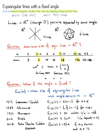
Lines Consider a line, a vector x 0 going from the origin to a point - PDF document

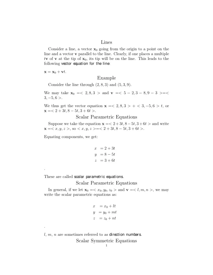
Lines Consider a line, a vector x 0 going from the origin to a point on the line and a vector v parallel to the line. Clearly, if one places a multiple t v of v at the tip of x 0 , its tip will be on the line. This leads to the following vector equation for the line : x = x 0 + v t . Example Consider the line through (2 , 8 , 3) and (5 , 3 , 9). We may take x 0 = < 2 , 8 , 3 > and v = < 5 − 2 , 3 − 8 , 9 − 3 > = < 3 , − 5 , 6 > . We thus get the vector equation x = < 2 , 8 , 3 > + < 3 , − 5 , 6 > t , or x = < 2 + 3 t, 8 − 5 t, 3 + 6 t > . Scalar Parametric Equations Suppose we take the equation x = < 2+3 t, 8 − 5 t, 3+6 t > and write x = < x, y, z > , so < x, y, z > = < 2 + 3 t, 8 − 5 t, 3 + 6 t > . Equating components, we get: = 2 + 3 t x y = 8 − 5 t = 3 + 6 t z . These are called scalar parametric equations . Scalar Parametric Equations In general, if we let x 0 = < x 0 , y 0 , z 0 > and v = < l, m, n > , we may write the scalar parametric equations as: x = x 0 + lt = y 0 + mt y z = z 0 + nt . l , m , n are sometimes referred to as direction numbers . Scalar Symmetric Equations 1

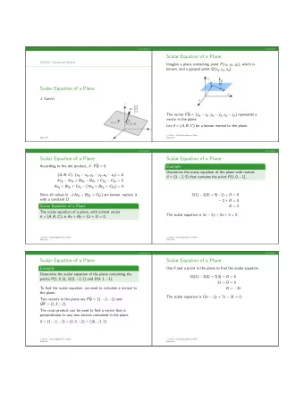
2 Suppose we take the scalar parametric equations x = 2 + 3 t = 8 − 5 t y z = 3 + 6 t . and solve each for t : x = 2 + 3 t , 3 t = x − 2, t = x − 2 3 . y = 8 − 5 t , − 5 t = y − 8, t = y − 8 − 5 . z = 3 + 6 t , 6 t = z − 3, t = z − 3 6 We can equate the values for t to get the scalar symmetric equations : = y − 8 x − 2 − 5 = z − 3 6 . 3 Scalar Symmetric Equations In general, the scalar symmetric equations are in the form: x − x 0 = y − y 0 = z − z 0 n . l m Relation to the Point-Slope Formula In two dimensions, the scalar symmetric equations are just a varia- tion of the Point-Slope Formula . If we take x − x 0 = y − y 0 and multiply both sides by m , we get m · x − x 0 = l m l y − y 0 , or y − y 0 = m l ( x − x 0 ). The quotient m l of the direction numbers is equal to the slope. Planes Consider a plane Π, a vector x 0 from the origin to a point in the plane, and a vector n perpendicular to the plane. We will refer to such a vector as a normal vector . Now consider a vector x from the origin to some point in the plane. The vector x − x 0 lies parallel to the plane and thus must be orthogonal to n . It follows that the dot product n · ( x − x 0 ) must equal 0. The equation n · ( x − x 0 ) is thus a vector equation for the plane . Alternatively, we may write n · x = n · x 0 .

3 Example Consider a plane containing the point (5 , 3 , 2) and normal vector n = < 4 , − 2 , 7 > . We may take x 0 = < 5 , 3 , 2 > , so its equation may be written < 4 , − 2 , 7 > · ( x − < 5 , 3 , 2 > ) = 0, or < 4 , − 2 , 7 > · x = < 4 , − 2 , 7 > · < 5 , 3 , 2 > , or < 4 , − 2 , 7 > · x = 28. Scalar Equation for a Plane Suppose we take the vector equation < 4 , − 2 , 7 > · x = 28 and let x = < x, y, z > , so < 4 , − 2 , 7 > · < x, y, z > = 28. We may multiply out the dot product to get 4 x − 2 y + 7 z = 28. In general, an equation of the form ax + by + cz = d will be an equation of a plane with normal vector < a, b, c > . Getting a Normal Vector If we have three points in a plane, we can take two vectors going between pairs of those points. Those vectors will be parallel to the plane, so their cross product will be orthogonal to the plane and may be taken as a normal vector. Example: Suppose a plane contains the points (1 , 5 , 3), (2 , 7 , 4), (4 , 8 , 6). We may take n = < 1 , 2 , 1 > × < 2 , 1 , 2 > = < 3 , 0 , − 3 > . We can make things a little simpler in this case, recognizing that any multiple of a normal vector is a normal vector, and taking n = < 1 , 0 , − 1 > instead. Quadric Surfaces The graphs of second degree polynomial equations in three vari- ables are called quadric surfaces . Sketching their graphs can be tricky. Sketches don’t have to be artistic, but need to be good enough to help visualize what the surface actually looks like. A key to sketching graphs is to sketch the traces in and/or parallel to the coordinate planes. We get these by setting one variable to be constant and seeing what the graph of the resulting equation is in the plane of the other two variables.

4 For example, if we set y to be constant, we get an equation in x and z and try to sketch its graph in the xz -plane. Its trace in R 3 is the curve congruent to that but shifted into a plane parallel to the xz -plane. Cylindrical Coordinates We get cylindrical coordinates by taking polar coordinates and sim- ply adding the z -coordinate. The coordinates of a point are therefore given by ( r, θ, z ). The relationship between rectangular and cylindrical coordinates is ba- sically the same as the one between rectangular coordinates and polar coordinates: x 2 + y 2 = r 2 x = r cos θ tan θ = y y = r sin θ x z = z z = z Graphs in Cylindrical Coordinates Cylindrical coordinates are useful for cylinders and cones, since their graphs are relatively simple. An equation of the form r = k gives a cylinder with radius k . An equation of the form z 2 = k · r 2 gives a cone. An equation of the form z = k · r 2 gives a paraboloid. Spherical Coordinates Spherical coordinates are another natural generalization of polar co- ordinates. • With spherical coordinates, the first coordinate ρ represents the distance of the point from the origin. • The second coordinate θ is the same as the second coordinate for cylindrical coordinates. • The third coordinate φ is the angle the ray from the origin to the point makes with the z -axis. The relationship between cylindrical and spherical coordinates is given by z = ρ cos φ , r = ρ sin φ . We can use the relationship between cylindrical and rectangular coor- dinates, particularly x = r cos θ and y = r sin θ , to see x = ρ sin φ cos θ , y = ρ sin φ sin θ , z = ρ cos φ . It’s also relatively obvious that ρ 2 = x 2 + y 2 + z 2 . Graphs in Spherical Coordinates

5 Spherical coordinates are particularly useful when dealing with spheres. Equations for certain planes and cones are also conveniently given in spherical coordinates. • The graph of ρ = k is a sphere of radius k . • The graph of θ = k is a plane through the z -axis, perpendicular to the xy -plane, making an angle k with the xz -plane. • The graph of φ = k is a cone through the origin where each line in the cone through the origin makes an angle k with the z -axis.