AM 205: lecture 13 Last time: ODE convergence and stability, - PowerPoint PPT Presentation

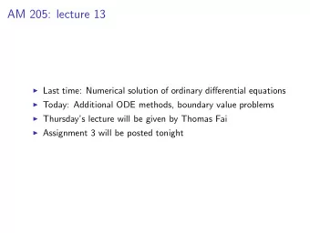
AM 205: lecture 13 ◮ Last time: ODE convergence and stability, Runge–Kutta methods ◮ Today: the Butcher tableau, multi-step methods, boundary value problems

Butcher tableau Can summarize an s + 1 stage Runge–Kutta method using a triangular grid of coefficients α 0 α 1 β 1 , 0 . . . . . . α s β s , 0 β s , 1 . . . β s , s − 1 γ 0 γ 1 . . . γ s − 1 γ s The i th intermediate step is i − 1 � f ( t k + α i h , y k + h β i , j k j ) . j =0 The ( k + 1)th answer for y is s � y k +1 = y k + h γ j k j . j =0

Estimation of error First approach: Richardson extrapolation. Suppose that y k +2 is the numerical result of two steps with size h of a Runge–Kutta method of order p , and w is the result of one big step with step size 2 h . Then the error of y k +2 can be approximated as y ( t k + 2 h ) − y k +2 = y k +2 − w + O ( h p +2 ) 2 p − 1 and y k +2 = y k +2 + y k +2 − w ˆ 2 p − 1 is an approximation of order p + 1 to y ( t 0 + 2 h ).

Estimation of error Second approach: can derive Butcher tableaus that contain an additional higher-order formula for estimating error. e.g. Fehlberg’s order 4(5) method, RKF45 0 1 1 4 4 3 3 9 8 32 32 12 1932 − 7200 7296 13 2197 2197 2197 439 3680 − 845 1 − 8 216 513 4104 1 − 8 − 3544 1859 − 11 2 2 27 2565 4104 40 25 1408 2197 − 1 y k +1 0 0 216 2565 4104 5 16 6656 28561 − 9 2 y k +1 ˆ 0 135 12825 56430 50 55 y k +1 is order 4 and ˆ y k +1 is order 5. Use y k +1 − ˆ y k +1 as an error estimate.

Higher-order methods Fehlberg’s 7(8) method 1 1 From Solving Ordinary Differential Equations by Hairer, Nørsett, and Wanner.

Stiff systems You may have heard of “stiffness” in the context of ODEs: an important, though somewhat fuzzy, concept Common definition of stiffness for a linear ODE system y ′ = Ay is that A has eigenvalues that differ greatly in magnitude 2 The eigenvalues determine the time scales, and hence large differences in λ ’s = ⇒ resolve disparate timescales simultaneously! 2 Nonlinear case: stiff if the Jacobian, J f , has large differences in eigenvalues, but this defn. isn’t always helpful since J f changes at each time-step

Stiff systems Suppose we’re primarily interested in the long timescale. Then: ◮ We’d like to take large time steps and resolve the long timescale accurately ◮ But we may be forced to take extremely small timesteps to avoid instabilities due to the fast timescale In this context it can be highly beneficial to use an implicit method since that enforces stability regardless of timestep size

Stiff systems From a practical point of view, an ODE is stiff if there is a significant benefit in using an implicit instead of explicit method e.g. this occurs if the time-step size required for stability is much smaller than size required for the accuracy level we want Example: Consider y ′ = Ay , y 0 = [1 , 0] T where � � 998 1998 A = − 999 − 1999 which has λ 1 = − 1, λ 2 = − 1000 and exact solution � 2 e − t − e − 1000 t � y ( t ) = − e − t + e − 1000 t

Multistep Methods So far we have looked at one-step methods, but to improve efficiency why not try to reuse data from earlier time-steps? This is exactly what multistep methods do: m m � � y k +1 = α i y k +1 − i + h β i f ( t k +1 − i , y k +1 − i ) i =1 i =0 If β 0 = 0 then the method is explicit We can derive the parameters by interpolating and then integrating the interpolant

Multistep Methods The stability of multistep methods, often called “zero stability,” is an interesting topic, but not considered here Question: Multistep methods require data from several earlier time-steps, so how do we initialize? Answer: The standard approach is to start with a one-step method and move to multistep once there is enough data Some key advantages of one-step methods: ◮ They are “self-starting” ◮ Easier to adapt time-step size

ODE Boundary Value Problems

ODE BVPs Consider the ODE Boundary Value Problem (BVP): 3 find u ∈ C 2 [ a , b ] such that − α u ′′ ( x ) + β u ′ ( x ) + γ u ( x ) = f ( x ) , x ∈ [ a , b ] for α, β, γ ∈ R and f : R → R The terms in this ODE have standard names: − α u ′′ ( x ): diffusion term β u ′ ( x ): convection (or transport) term γ u ( x ): reaction term f ( x ): source term 3 Often called a “Two-point boundary value problem”

ODE BVPs Also, since this is a BVP u must satisfy some boundary conditions, e.g. u ( a ) = c 1 , u ( b ) = c 2 u ( a ) = c 1 , u ( b ) = c 2 are called Dirichlet boundary conditions Can also have: ◮ A Neumann boundary condition: u ′ ( b ) = c 2 ◮ A Robin (or “mixed”) boundary condition: 4 u ′ ( b ) + c 2 u ( b ) = c 3 4 With c 2 = 0, this is a Neumann condition

ODE BVPs This is an ODE, so we could try to use the ODE solvers from III.3 to solve it! Question: How would we make sure the solution satisfies u ( b ) = c 2 ?

ODE BVPs Answer: Solve the IVP with u ( a ) = c 1 and u ′ ( a ) = s 0 , and then update s k iteratively for k = 1 , 2 , . . . until u ( b ) = c 2 is satisfied This is called the “shooting method”, we picture it as shooting a projectile to hit a target at x = b (just like Angry Birds!) However, the shooting method does not generalize to PDEs hence it is not broadly useful