All in one Reporting with RStudio (slides) Presentation December - PDF document
See discussions, stats, and author profiles for this publication at: https://www.researchgate.net/publication/313221458 All in one Reporting with RStudio (slides) Presentation December 2016 CITATIONS READS 0 209 1 author: Satu Helske
See discussions, stats, and author profiles for this publication at: https://www.researchgate.net/publication/313221458 All in one – Reporting with RStudio (slides) Presentation · December 2016 CITATIONS READS 0 209 1 author: Satu Helske University of Turku 16 PUBLICATIONS 97 CITATIONS SEE PROFILE Some of the authors of this publication are also working on these related projects: Multigenerational Demography View project Hidden Markov modelling for complex social sequence data View project All content following this page was uploaded by Satu Helske on 02 February 2017. The user has requested enhancement of the downloaded file.
All in one Reporting with RStudio Satu Helske 8 December 2016
Learning R ◮ Online courses ◮ Lynda ◮ DataCamp ◮ Code School ◮ Books ◮ Getting used to R, RStudio, and R Markdown by Chester Ismay ◮ R for Data Science by Garrett Grolemund and Hadley Wickham ◮ R for Stata Users by Robert A. Muenchen and Joseph M. Hilbe
Rstudio ◮ Open source graphical interface for R and related tools ◮ Code completion, syntax highlighting, code diagnostics ◮ Autosave, command history, plotting history, environment browser, integrated searchable help ◮ R projects for easy return to and switching between jobs ◮ https://www.rstudio.com/
Reporting with knitr
What? ◮ Mix text, R code, R output, R graphics, mathematics ◮ Notes, reports, exercises, slides, research papers ◮ PDF, Word, html etc.
Why? ◮ Reproducible research ◮ Change in data → Change in report ◮ Sharing work with others ◮ Easier to adjust font sizes in figures ◮ No copy-paste errors
How? ◮ knitr with R Markdown ◮ Simple, fast ◮ Limited functionalities ◮ Rmd file ◮ knitr with LaTeX ◮ Precice control ◮ Requires LaTeX skills ◮ Rnw file
R Markdown
R Markdown ◮ Simple formatting syntax ◮ Fully reproducible documents ◮ Closely integrated to Rstudio ◮ Based on Markdown language, knitr , and pandoc ◮ http://rmarkdown.rstudio.com/
Workflow
Open R Markdown file
Write
Add R code
Render
Markdown syntax
YAML header --- title: All in one subtitle: RStudio for reporting author: Satu Helske date: 8 December 2016 output: ioslides_presentation ---
Headers # Header 1 ## Header 2 ### Header 3
Typesetting examples ◮ _italics_ or *italics* produces italics ◮ __bold__ or **bold** produces bold ◮ superscriptˆ2ˆ produces superscript 2 ◮ subscripts~2~ produces subscripts 2
Lists - Item 1 + Item A * Item B - Item 2 produces ◮ Item 1 ◮ Item A ◮ Item B ◮ Item 2 (-, +, and * are equivalents)
Tables Type | Freq | % ---------| ------|----- Apples | 7 | 44 Oranges | 9 | 56 produces Type Freq % Apples 7 44 Oranges 9 56
Mathematics Mathematics like in LaTex: y_i = \beta_0 + \beta_1 x_i + \epsilon_i produces y i = β 0 + β 1 x i + ǫ i
Embedding R code
Code chunks ◮ Start with three backticks followed by {r} ◮ Optional own chunk name (unique, no spaces or periods) ◮ Optional options (R expressions) ◮ R code in between ◮ End with three backticks
Some options for code chunks ◮ eval : run R code ( TRUE / FALSE ) ◮ echo : show R code in output ◮ warning , error , message : show warnings/errors/messages in output ◮ cache : save objects ◮ chunk only evaluated 1st time, later objects are loaded ◮ fig.width , fig.height , fig.asp : settings for figure size ◮ fig.cap : caption for figure
Dynamic tables library (knitr) regression_table <- lm (dist ~ speed, data = cars) kable ( summary (regression_table)$coefficients, digits = c (2, 2, 2, 3)) Estimate Std. Error t value Pr(>|t|) (Intercept) -17.58 6.76 -2.60 0.012 speed 3.93 0.42 9.46 0.000
Figures plot (cars) 120 100 80 dist 60 40 20 0 5 10 15 20 25 speed
Dynamic code within text The sample size was `r nrow(cars)`. The average distance that was travelled was `r mean(cars$dist)`. produces The sample size was 50. The average distance that was travelled was 42.98.
Writing papers
Bookdown ◮ R package built on top of R Markdown ◮ Book or “book” from several R Markdown documents ◮ Numbering, cross-referencing, appendices ◮ Output options (YAML) ◮ bookdown::html_document2 ◮ bookdown::word_document2 ◮ bookdown::pdf_book ◮ https://bookdown.org/yihui/bookdown/
Abstract Option abstract in YAML --- title: All in one - RStudio for reporting author: Satu Helske output: pdf_document abstract: "This is my abstract." ---
Numbers and cross-references ◮ Use bookdown outputs (e.g., bookdown::pdf_document2 ) ◮ Figures ◮ Name chunk (e.g., my-plot ), fig.cap in R chunk options ◮ Cross-reference in text: \@ref(fig:my-plot) ◮ Tables ◮ Name chunk (e.g., my-table ) ◮ kable function in knitr ; add caption argument ◮ Cross-reference: \@ref(tab:my-table) ◮ Sections ◮ Add {#my-section} after section header ◮ Cross-reference: \@ref(my-section)
Bibliographies ◮ BibTeX bibliographies (.bib) recommended @Book{Author2015, author = {Author, Alice and Writer, William}, title = {Book of something}, publisher = {Publisher P}, year = {2015}, address = {City, Country} } ◮ Add bibliography + options in YAML, e.g. --- bibliography: my_bibliography.bib biblio-style: apalike link-citations: true ---
Citing ◮ Citing in text: @Author2015 ◮ Citing in brackets: [@Author2015; @Writer2016] ◮ References printed at the end of the document → Last line is section header, e.g. # References
LaTeX
knitr with LaTeX ◮ Normal LaTeX with embedded R code ◮ Inline code: \Sexpr{} ◮ Code chunks: <<my_cars_plot, fig.height=6, fig.width=8>>= plot(cars) @
Open Rnw document
Before rendering with knitr ◮ Change RStudio default from Sweave to knitr
Rendering
Tips ◮ When writing, use html output ◮ Fast to render ◮ No need to worry about pages, margins etc. ◮ Cache time-consuming code chunks with the cache option ◮ Note: cached chunks only change if you change the contents → Subsequent chunks do not automatically change (unless cache cleared) ◮ For data cleaning, manipulation, and visualization, see tidyverse ◮ Finding help ◮ Stack overflow ◮ Github project pages
Tips for collaboration ◮ Share the Rmd (R Markdown) file ◮ Use commenting (Crtl + Shift + C) to suggest changes or to show where you have modified the file ◮ Share the Word file ◮ Use the commenting options in Word ◮ Copy and paste changes into the Rmd file ◮ Use version control such as Git ◮ Integrated in RStudio ◮ Automatically keeps track of all changes in all previous versions ◮ Might be a steep learning curve, but for small projects learning the very basics is usually enough ◮ Learn (enough) Git in 15 minutes: https://try.github.io
Useful links ◮ R Markdown cheat sheet by RStudio ◮ knitr in a knutshell by Karl Broman ◮ knitr by Yihui Xie ◮ LaTeX by the LaTeX Project ◮ Citing ◮ BibTex by Martin J. Osborne ◮ Bibliographies and citations by Rstudio ◮ Citing with Mendeley by Rosanna van Hespen ◮ Tables ◮ Precise control: xtables by David B. Dahl, David Scott, Jonathan Swinton and others ◮ Good-looking tables with minimal effort, e.g., summarizing multiple models: stargazer by Marek Hlavac View publication stats View publication stats
Recommend
More recommend
Explore More Topics
Stay informed with curated content and fresh updates.



![MARKDOWN SLIDES [EN] MARKDOWN SLIDES [EN] MARKDOWN SLIDES [EN] MARKDOWN SLIDES [EN] MARKDOWN](https://c.sambuz.com/818511/markdown-slides-en-markdown-slides-en-markdown-slides-en-s.webp)

