A Study of Probability Estimation Techniques for Rule Learning - PowerPoint PPT Presentation
A Study of Probability Estimation Techniques for Rule Learning Jan-Nikolas Sulzmann Johannes F urnkranz September 7, 2009 | KE TUD | Sulzmann & F urnkranz | 1 KE Outline Motivation Rule Learning and Probability Estimation
A Study of Probability Estimation Techniques for Rule Learning Jan-Nikolas Sulzmann Johannes F¨ urnkranz September 7, 2009 | KE TUD | Sulzmann & F¨ urnkranz | 1 KE
Outline Motivation Rule Learning and Probability Estimation Probabilistic Rule Learning Basic Probability Estimation Shrinkage Rule Learning Algorithm Experiments Conclusions & Future Work September 7, 2009 | KE TUD | Sulzmann & F¨ urnkranz | 2 KE
Motivation ◮ In many pratical applications a strict classification is insufficient ◮ Provide a confidence score ◮ Rank by class probability → Predict a class probability distribution ◮ Na¨ ıve approach: Precision ◮ Extreme probability estimates for rules covering few examples → Probability estimates need to be smoothed ◮ Previous work on Probability Estimation Trees (PETs) ◮ m-Estimate & Laplace-estimate work well on PETs ◮ Unpruned trees work better for probability estimation than pruned ones ◮ Investigated Shrinkage on PETs ◮ How does these techniques behave on probabilistic rules? September 7, 2009 | KE TUD | Sulzmann & F¨ urnkranz | 3 KE
Conjunctive Rule Mining Conjunctive rule: condition 1 ∧ · · · ∧ condition | r | ⇒ class ◮ | r | : size of the rule A ◮ r k : subrule of r consists of the first k conditions ◮ r ⊇ x : the rule r covers the instance x , if x meets all conditions of r Probabilistic rule: ◮ Extension: class probability distribution ◮ Pr( c | r ⊇ x ): probability that an instance x covered by rule r belongs to c September 7, 2009 | KE TUD | Sulzmann & F¨ urnkranz | 4 KE
Basic Probability Estimation Smoothing methods: ıve ( c | r k ⊇ x ) = n c Na¨ ıve approach/Precision (Na¨ ıve): Pr Na¨ r n r n c r +1 Laplace-estimate (Laplace): Pr Laplace ( c | r k ⊇ x ) = n r + | C | Pr m ( c | r k ⊇ x ) = n c r + m · Pr( c ) m-estimate (m): n r + m Note: ◮ | C | : number of classes ◮ n r : instances covered by the rule r ◮ n c r : instances belonging to class c covered by the rule r ◮ Pr( c ): a priori probability of class c September 7, 2009 | KE TUD | Sulzmann & F¨ urnkranz | 5 KE
Shrinkage Basic Idea: Weighted sum of the probability distributions of the sub rules | r | � w k Shrink ( c | r ⊇ x ) = Pr c · Pr( c | r k ⊇ x ) k =0 Calculating the weights: ◮ Smoothing the probabilities: Consequently remove an example Smoothed ( c | r k ⊇ x ) = n c − ( c | r k ⊇ x ) + n r − n c r r Pr · Pr · Pr + ( c | r k ⊇ x ) n r n r ◮ Normalization: Pr Smoothed ( c | r k ⊇ x ) w k c = � | r | i =0 Pr Smoothed ( c | r i ⊇ x ) September 7, 2009 | KE TUD | Sulzmann & F¨ urnkranz | 6 KE
Ripper: Generation modes Ordered Mode ◮ Ordered class binarization: ◮ Classes ordered by their frequency ◮ The rules are learned separately for each class in this order ◮ Each class vs. more frequent classes ( c i vs. c i +1 , ..., c n ) ◮ No rules for the most frequent class, except for a default rule ◮ Decision list: rules are ordered by the order they are learned Unordered Mode ◮ Unordered/One-against-all class binarization ◮ Voting scheme: ◮ Select for each class the covering rule(s) ◮ Use the most confident rule for prediction ◮ Tie breaking: more frequent class September 7, 2009 | KE TUD | Sulzmann & F¨ urnkranz | 7 KE
Rule Learning Algorithm Training: employed JRip, the Weka implementation of Ripper ◮ Only ordered mode supported, unordered mode reimplemented ◮ Other minor modifications for the probability estimation (e.g. statistical counts of sub rules) ◮ Incremental reduced error pruning can be turned on/off ◮ MDL-based post pruning cannot be turned off Classification: selecting the most probable class ◮ Determine all covering rules for a given test instance ◮ Select the most probable class of each rule ◮ Use this class value for prediction and the class probability for comparison ◮ No covering rule, use the class distribution of the default rule September 7, 2009 | KE TUD | Sulzmann & F¨ urnkranz | 8 KE
Experimental Setup Data: ◮ 33 data sets of the UCI repository Setup: ◮ 4 configurations of Ripper: (un-)ordered mode and (no) pruning ◮ Probability estimation techniques: ◮ Na¨ ıve/Precision, Laplace, m -estimate ( m ∈ { 2, 5, 10 } ) ◮ Used stand-alone (B) or in combination with shrinkage (S) Evaluation: ◮ Stratified 10-fold cross validation using weighted AUC ◮ Friedman test with a post-hoc Nemenyi test (Demsar): significance 95% ◮ For all comparisons Friedman test rejected the equality of the methods September 7, 2009 | KE TUD | Sulzmann & F¨ urnkranz | 9 KE
Ordered Rule Sets without Pruning ◮ 2 good choices, m-Estimate ( m ∈ { 2, 5 } ) used stand-alone ◮ Both Precision techniques rank in the lower half ◮ JRip is positioned in the lower third → Probability estimation techniques improves over the default JRip ◮ Shrinkage is outperformed by the stand-alone techniques (except Precision) September 7, 2009 | KE TUD | Sulzmann & F¨ urnkranz | 10 KE
Ordered Rule Sets with Pruning ◮ Best group: all stand-alone methods and JRip ◮ JRip dominates this group ◮ All stand-alone methods rank for their shrinkage → Shrinkage is not advisable September 7, 2009 | KE TUD | Sulzmann & F¨ urnkranz | 11 KE
Unordered Rule Sets without Pruning ◮ Best group: all stand-alone methods (except Precision) and the m-estimates with m = 5 and m = 10 and shrinkage ◮ JRip belongs to the worst group ◮ Shrinkage methods are outperformed by their stand-alone counterparts September 7, 2009 | KE TUD | Sulzmann & F¨ urnkranz | 12 KE
Unordered Rule Sets with Pruning ◮ Best group: all stand-alone methods and the m-estimates with m = 5 and m = 10 and shrinkage ◮ The shrinkage methods are outperformed by their stand-alone counterparts ◮ JRip is the worst choice September 7, 2009 | KE TUD | Sulzmann & F¨ urnkranz | 13 KE
Pruned vs. Unpruned Rule Sets Jrip Precision Laplace M 2 M 5 M 10 Win 26 23 19 20 19 18 20 19 20 19 20 Loss 7 10 14 13 14 15 13 14 13 14 13 Win 26 21 9 8 8 8 8 8 8 8 6 Loss 7 12 24 25 25 25 25 25 25 25 27 Table: Win/loss for ordered rule sets (top) and unordered rule sets (bottom) ◮ Mixed Results for Pruning ◮ Improved the results of the ordered approach ◮ Worsened the results of the unordered approach → Contrary to PETs, rule pruning is not always a bad choice ◮ Examples not covered by a rule are classified with default rule ◮ Prune complete rule: more examples classified with default rule ◮ Prune conditions: less examples classified with default rule September 7, 2009 | KE TUD | Sulzmann & F¨ urnkranz | 14 KE
Conclusions & Future Work Conclusions ◮ JRip can be improved by simple estimation techniques ◮ Unordered rule induction should be preferred for probabilistic classification ◮ m-estimate typically outperformed the other methods ◮ Shrinkage did not improve the probability estimation in general ◮ Contrary to PETs pruning is not always a bad choice Future Work ◮ Previous work: Lego-Framework for class association rules ◮ Using the framework for the generation of probabilistic rules ◮ Investigating the performance of generation and selection September 7, 2009 | KE TUD | Sulzmann & F¨ urnkranz | 15 KE
Recommend
More recommend
Explore More Topics
Stay informed with curated content and fresh updates.
