Single-parameter models: Gaussian (normal) data Applied Bayesian - PowerPoint PPT Presentation
Single-parameter models: Gaussian (normal) data Applied Bayesian Statistics Dr. Earvin Balderama Department of Mathematics & Statistics Loyola University Chicago September 19, 2017 The Gaussian (normal) model 1 Last edited September 8,
Single-parameter models: Gaussian (normal) data Applied Bayesian Statistics Dr. Earvin Balderama Department of Mathematics & Statistics Loyola University Chicago September 19, 2017 The Gaussian (normal) model 1 Last edited September 8, 2017 by Earvin Balderama <ebalderama@luc.edu>
One-parameter models The normal model The Gaussian (normal) distribution is possibly the most useful (or most utilized) model in data analyses. Y ∼ Normal ( µ, σ 2 ) Y ∈ ( −∞ , ∞ ) E ( Y ) = µ V ( Y ) = σ 2 If we choose a normal model for our likelihood function, there are two parameters to estimate. However, we can break up the task into 2 one-parameter models by: Estimating the mean , assuming the variance is known. 1 Estimating the variance , assuming the mean is known. 2 The Gaussian (normal) model 2 Last edited September 8, 2017 by Earvin Balderama <ebalderama@luc.edu>
One-parameter models Estimating µ - Likelihood Suppose we have n independent and identically distributed Gaussian observations Y 1 , . . . , Y n . Given a mean µ and (known) variance σ 2 , the distribution of each Y i is Y i | µ, σ 2 iid ∼ Normal ( µ, σ 2 ) Thus, the likelihood function for Y 1 = y 1 , . . . , Y n = y n is n � � 2 � 1 − 1 � y i − µ � f ( y 1 , . . . , y n | µ, σ 2 ) = √ exp 2 σ 2 πσ i = 1 � n � n � � 1 − 1 ( y i − µ ) 2 � = √ exp 2 σ 2 2 πσ i = 1 The Gaussian (normal) model 3 Last edited September 8, 2017 by Earvin Balderama <ebalderama@luc.edu>
One-parameter models Estimating µ - Prior µ is the parameter of interest, and is continuous over the entire real line. A natural prior distribution to select would then be µ | σ 2 ∼ Normal ( θ, τ 2 ) . To make the math easier to interpret later on, simply let τ 2 = σ 2 m . µ | σ 2 ∼ Normal � � θ, σ 2 , m where the prior mean θ is the best guess before we observe data, and the prior variance σ 2 m (via m > 0) controls the strength of the prior. Note: How to choose m ? The Gaussian (normal) model 4 Last edited September 8, 2017 by Earvin Balderama <ebalderama@luc.edu>
One-parameter models Estimating µ - Posterior We can now derive the posterior distribution, which happens to be: � n ¯ σ 2 y + m θ � µ | y 1 , . . . , y n , σ 2 ∼ Normal n + m , n + m The Gaussian (normal) model 5 Last edited September 8, 2017 by Earvin Balderama <ebalderama@luc.edu>
One-parameter models Estimating µ - Shrinkage The prior mean was E ( µ | σ 2 ) = θ . The posterior mean is µ B = E ( µ | y 1 , . . . , y n , σ 2 ) = n ¯ y + m θ ˆ n + m � n � � m � ¯ = y + θ n + m n + m The posterior mean is between the sample mean ¯ y and the prior mean θ . µ B close to the sample mean ¯ When is ˆ y ? small m 1 When is ˆ µ B shrunk towards the prior mean θ ? large m 2 The Gaussian (normal) model 6 Last edited September 8, 2017 by Earvin Balderama <ebalderama@luc.edu>
One-parameter models Estimating µ - Shrinkage The prior variance was V ( µ | σ 2 ) = σ 2 m . The posterior variance is σ 2 V ( µ | y 1 , . . . , y n , σ 2 ) = n + m Note: Recall the sampling variance of ¯ Y is σ 2 n . m can thus be loosely interpreted as the “ prior number of observations .” The Gaussian (normal) model 7 Last edited September 8, 2017 by Earvin Balderama <ebalderama@luc.edu>
One-parameter models Estimating σ 2 - Likelihood Suppose we have n independent and identically distributed Gaussian observations Y 1 , . . . , Y n . Given a variance σ 2 and (known) mean µ , the distribution of each Y i is Y i | µ, σ 2 iid ∼ Normal ( µ, σ 2 ) Thus, the likelihood function for Y 1 = y 1 , . . . , Y n = y n is n � � 2 � 1 − 1 � y i − µ � f ( y 1 , . . . , y n | µ, σ 2 ) = √ exp 2 σ 2 πσ i = 1 � n � n � � 1 − 1 ( y i − µ ) 2 � = √ exp 2 σ 2 2 πσ i = 1 The Gaussian (normal) model 8 Last edited September 8, 2017 by Earvin Balderama <ebalderama@luc.edu>
One-parameter models Estimating σ 2 - Prior σ 2 is the parameter of interest, and is continuous over ( 0 , ∞ ) . So, naturally, we would want to select the prior distribution σ 2 | µ ∼ Gamma ( a , b ) . The Gaussian (normal) model 9 Last edited September 8, 2017 by Earvin Balderama <ebalderama@luc.edu>
One-parameter models Estimating σ 2 - Prior σ 2 is the parameter of interest, and is continuous over ( 0 , ∞ ) . So, naturally, we would want to select the prior distribution σ 2 | µ ∼ Gamma ( a , b ) . However, the gamma prior is not conjugate for the normal variance. 1 The gamma prior is conjugate for the precision , σ 2 . Thus, the math is easier if we use: � 1 � µ ∼ Gamma ( a , b ) , � σ 2 which implies σ 2 | µ ∼ InverseGamma ( a , b ) , and the PDF for inverse gamma is b a f ( σ 2 | µ ) = σ 2 � − a − 1 e − b /σ 2 � Γ( a ) The Gaussian (normal) model 9 Last edited September 8, 2017 by Earvin Balderama <ebalderama@luc.edu>
One-parameter models Estimating σ 2 - Posterior We can now derive the posterior distribution, which happens to be: � n 2 + a , SSE � σ 2 � � y 1 , . . . , y n , µ ∼ InverseGamma + b , � 2 n � ( y i − µ ) 2 . where the sum of squared errors SSE = i = 1 The Gaussian (normal) model 10 Last edited September 8, 2017 by Earvin Balderama <ebalderama@luc.edu>
One-parameter models Estimating σ 2 - Shrinkage The prior mean (if it exists, i.e., for a > 1) was E ( σ 2 | µ ) = b a − 1 . The posterior mean is SSE + b E ( σ 2 | y 1 , . . . , y n , µ ) = 2 n 2 + a − 1 = SSE + b n + 2 a − 2 It is common to take a and b to be small to give an uninformative prior, ⇒ so that the posterior mean approximates the sample variance SSE n − 1 . = The Gaussian (normal) model 11 Last edited September 8, 2017 by Earvin Balderama <ebalderama@luc.edu>
Recommend
More recommend
Explore More Topics
Stay informed with curated content and fresh updates.
