A graphical approach to sequentially rejective multiple test - PowerPoint PPT Presentation
A graphical approach to sequentially rejective multiple test procedures Martin Posch Center for Medical Statistics, Informatics and Intelligent Systems Medical University of Vienna Joint work with Frank Bretz, Willi Maurer, Werner Brannath
A graphical approach to sequentially rejective multiple test procedures Martin Posch Center for Medical Statistics, Informatics and Intelligent Systems Medical University of Vienna Joint work with Frank Bretz, Willi Maurer, Werner Brannath µ Toss, Berlin 2010
Sequentially rejective, weighted Bonferroni type tests • Applied in clinical trials with multiple treatment arms, subgroups and endpoints • Bonferroni-Holm Test, Fixed Sequence Test, Fallback Test, Gatekeeping Tests, ... • Allow to map the difference in importance as well as the relationship between research questions onto the multiple test procedure. • However: The testing procedure can be technical and often hard to communicate. Parallell gatekeeping: Testing F 1 = { H 1 , H 2 } , F 2 = { H 3 , H 4 } Rejection of hypotheses in the family F 2 = { H 3 , H 4 } is only of interest if at least one of the hypotheses in the family F 1 = { H 1 , H 2 } can be rejected
Parallel Gatekeeping (Dmitrienko, Offen & Westfall, 2003)
Heuristics Notation • H 1 , . . . , H m : m null hypotheses. • p 1 , . . . , p m : m elementary p-values • α = ( α 1 , . . . , α m ) : initial allocation of the type I error rate α = � m i = 1 α i . “ α Reshuffling” 1 If a hypothesis H i can be rejected at level α i , reallocate its level to one of the other hypotheses (according to a prefixed rule) 2 Repeat the testing with the resulting α levels. 3 Go to step 1 until no hypothesis can be rejected anymore. Does this lead to a FWE-controlling test?
Example: Bonferroni-Holm Test α α 1 2 2 H 1 H 2 1
Example: Bonferroni-Holm Test ( α = 0 . 025) α α 1 2 2 H 1 H 2 p 1 = 0 . 04 p 2 = 0 . 01 1
Example: Bonferroni-Holm Test ( α = 0 . 025) α α 1 2 2 H 1 H 2 p 1 = 0 . 04 p 2 = 0 . 01 1
Example: Bonferroni-Holm Test ( α = 0 . 025) 1 α H 1 H 2 p 1 = 0 . 04 1
Example: Bonferroni-Holm Test ( α = 0 . 025) α H 1 p 1 = 0 . 04
Example: Parallel Gatekeeping α α 2 2 H 1 H 2 1 / 2 1 / 2 1 / 2 1 / 2 1 H 3 H 4 0 0 1 To the procedure of Dmitrienko et al. (2003)
Example: Parallel Gatekeeping ( α = 0 . 025) α α 2 2 H 1 H 2 p 1 = 0 . 01 p 2 = 0 . 005 1 / 2 1 / 2 1 / 2 1 / 2 1 H 3 H 4 p 3 = 0 . 001 p 4 = 0 . 04 0 0 1 .
Example: Parallel Gatekeeping ( α = 0 . 025) α α 2 2 H 1 H 1 H 2 p 1 = 0 . 01 p 2 = 0 . 005 1 / 2 1 / 2 1 / 2 1 / 2 1 H 3 H 4 p 3 = 0 . 001 p 4 = 0 . 04 0 0 1 .
Example: Parallel Gatekeeping ( α = 0 . 025) α α 2 2 H 1 H 1 H 2 p 1 = 0 . 01 p 2 = 0 . 005 1 / 2 1 / 2 1 / 2 1 / 2 1 / 2 1 / 2 1 H 3 H 4 p 3 = 0 . 001 p 4 = 0 . 04 0 0 1 .
Example: Parallel Gatekeeping ( α = 0 . 025) α 2 H 1 H 1 H 2 p 2 = 0 . 005 1 / 2 1 / 2 1 / 2 1 / 2 1 / 2 1 / 2 1 H 3 H 4 p 3 = 0 . 001 p 4 = 0 . 04 α α 1 4 4 .
Example: Parallel Gatekeeping ( α = 0 . 025) α 2 H 2 p 2 = 0 . 005 1 / 2 1 / 2 1 H 3 H 4 p 3 = 0 . 001 p 4 = 0 . 04 α α 1 4 4 .
Example: Parallel Gatekeeping ( α = 0 . 025) α 2 H 2 p 2 = 0 . 005 1 / 2 1 / 2 1 H 3 H 3 H 4 p 3 = 0 . 001 p 4 = 0 . 04 α α 1 4 4 .
Example: Parallel Gatekeeping ( α = 0 . 025) α 2 H 2 p 2 = 0 . 005 1 / 2 1 / 2 1 H 3 H 3 H 4 p 4 = 0 . 04 α 1 2 .
Example: Parallel Gatekeeping ( α = 0 . 025) α 2 H 2 p 2 = 0 . 005 1 H 4 p 4 = 0 . 04 α 2 .
Example: Parallel Gatekeeping ( α = 0 . 025) α 2 H 2 p 2 = 0 . 005 1 H 4 p 4 = 0 . 04 α 2 .
Example: Parallel Gatekeeping ( α = 0 . 025) H 4 p 4 = 0 . 04 α .
General Definition of the Multiple Test Procedure General definition of the multiple test • α = ( α 1 , . . . , α m ) , � m i = 1 , α i = α , initial levels • G = ( g ij ) : m × m transition matrix g ij with 0 ≤ g ij ≤ 1, g ii = 0 and � m j = 1 g ij ≤ 1 for all i = 1 , . . . , m . • g ij . . . fraction of the level of H i that is allocated to H j . • G and α determine the graph and the multiple test.
The Testing Procedure Set J = { 1 , . . . , m } . 1 Select a j such that p j ≤ α j . If no such j exists, stop, otherwise reject H j . 2 Update the graph: J → J / { j } � α ℓ + α j g j ℓ , ℓ ∈ J α ℓ → 0 , otherwise � g ℓ k + g ℓ j g jk ℓ, k ∈ J , ℓ � = k 1 − g ℓ j g j ℓ , g ℓ k → 0 , otherwise 3 Go to step 1.
The Testing Procedure Set J = { 1 , . . . , m } . 1 Select a j such that p j ≤ α j . If no such j exists, stop, otherwise reject H j . 2 Update the graph: J → J / { j } � α ℓ + α j g j ℓ , ℓ ∈ J α ℓ → 0 , otherwise � g ℓ k + g ℓ j g jk ℓ, k ∈ J , ℓ � = k 1 − g ℓ j g j ℓ , g ℓ k → 0 , otherwise 3 Go to step 1.
The Testing Procedure Set J = { 1 , . . . , m } . 1 Select a j such that p j ≤ α j . If no such j exists, stop, otherwise reject H j . 2 Update the graph: J → J / { j } � α ℓ + α j g j ℓ , ℓ ∈ J α ℓ → 0 , otherwise � g ℓ k + g ℓ j g jk ℓ, k ∈ J , ℓ � = k 1 − g ℓ j g j ℓ , g ℓ k → 0 , otherwise 3 Go to step 1.
Updating the Graph H 2 H 2 g 12 g 23 g 13 H 1 H 3
Updating the Graph H 2 g 12 g 23 g 13 + g 12 g 23 H 1 H 3
Updating the Graph H 2 H 2 g 12 g 23 g 21 g 13 H 1 H 3
Updating the Graph H 2 g 12 g 23 g 21 g 12 g 21 g 13 + g 12 g 23 H 1 H 3
Updating the Graph H 2 g 12 g 23 g 21 g 12 g 21 g 13 + g 12 g 23 1 − g 12 g 21 H 1 H 3
Control of the FWE Theorem The initial levels α , the transition matrix G and the algorithm define a unique multiple testing procedure controlling strongly the FWER at level α . Proof: • The graph and algorithm define weighted Bonferroni tests for all intersection hypotheses. • The algorithm is a short cut for the resulting closed test.
Closed Testing with Weighted Bonferroni Tests Closed Testing Procedure: 1 Define level α tests for all intersection hypotheses H J = ∩ i ∈ J H i , J ⊆ { 1 , . . . , m } . 2 Reject H j , at multiple level α , if for all J ⊆ { 1 , . . . , m } that contain j the intersection hypotheses H J can be rejected at level α . Weighted Bonferroni Test. 1 For each J ⊆ { 1 , . . . , m } define α J j ∈ J α J j such that � j = α . 2 Reject H J , if p j ≤ α J j for some j ∈ J .
Fixed Sequence Test 0 1 0 G = α = ( α, 0 , 0 ) , 0 0 1 0 0 0 α 0 0 1 1 H 1 H 2 H 3
Fallback Procedure (Wiens, 2003) 0 1 0 G = α = ( α 1 , α 2 , α 3 ) , 0 0 1 0 0 0 α 1 α 2 α 3 1 1 H 1 H 2 H 3
Improved Fallback Procedure (Wiens & Dmitrienko, 2005) 0 1 0 G = α = ( α 1 , α 2 , α 3 ) , 0 0 1 1 / 2 1 / 2 0 α 1 α 2 α 3 1 1 H 1 H 2 H 3 1/2 1/2
Yet another improved Fallback Procedure 0 1 0 G = α = ( α 1 , α 2 , α 3 ) , 1 − ǫ 0 ǫ 1 0 0 α 1 α 2 α 3 1 ǫ H 1 H 2 H 3 1 − ǫ 1 Let ǫ → 0, see explanation below.
Shifting level between families of hypotheses (1) 1 α/ 2 α/ 2 H 1 H 2 1 1 H 3 0 Test strategy • H 1 , H 2 tested with Bonferroni-Holm • H 3 tested (at level α ) only if H 1 and H 2 are rejected
Shifting level between families of hypotheses (2) 0 1 − ǫ ǫ � α G = 2 , α � α = 2 , 0 , 1 − ǫ 0 ǫ 0 0 0 1 − ǫ α/ 2 α/ 2 H 1 H 2 1 − ǫ ǫ ǫ H 3 0 Let ǫ → 0.
Shifting level between families of hypotheses (2) 1 − ǫ α/ 2 α/ 2 H 1 H 2 1 − ǫ ǫ ǫ H 3 0 Let ǫ → 0.
Shifting level between families of hypotheses (2) 1 − ǫ α H 1 H 2 1 − ǫ ǫ ǫ H 3 0 Let ǫ → 0.
Shifting level between families of hypotheses (2) 0 0 1 G = α = ( α, 0 , 0 ) , 0 0 0 0 0 0 α H 1 1 H 3 0 Let ǫ → 0.
Parallel Gatekeeping (Dmitrienko, Offen & Westfall, 2003) 0 0 0 . 5 0 . 5 0 0 0 . 5 0 . 5 G = � α 2 , α � α = 2 , 0 , 0 , 0 0 0 1 0 0 1 0 α α 2 2 H 1 H 2 1 / 2 1 / 2 1 / 2 1 / 2 1 H 3 H 4 0 0 1
Improved Parallel Gatekeeping (Hommel, Bretz & Maurer, 2007) 0 0 0 . 5 0 . 5 0 0 0 . 5 0 . 5 G = � α 2 , α � α = 2 , 0 , 0 , ǫ 0 0 1 − ǫ 0 ǫ 1 − ǫ 0 α α 2 2 H 1 H 2 1 / 2 1 / 2 ǫ 1 / 2 1 / 2 ǫ 1 − ǫ H 3 H 4 0 0 1 − ǫ
When is a graph complete? ... and cannot be improved by adding additional edges? A sufficient condition for completeness: • the weights of outgoing edges sum to one at each node and • every node is accessible from any of the other nodes If α i > 0 , i = 1 , . . . , m , this is also a necessary condition for completeness.
How general is the procedure? Can all consonant closed test procedures using weighted Bonferroni Tests for the intersection hypotheses be constructed with the graphical procedure? No: • For the general procedure we can choose weights for 2 m − 1 intersection hypotheses. • The graphical procedure is defined by m 2 + m parameters.
Extensions • Multiplicity adjusted confidence bounds (Guilbaud (2008) and Strassburger and Bretz (2008)) • Adjusted p-values
Recommend
More recommend
Explore More Topics
Stay informed with curated content and fresh updates.
