6.2 Bump Mapping & Clipping Hao Li http://cs420.hao-li.com 1 - PowerPoint PPT Presentation
Fall 2018 CSCI 420: Computer Graphics 6.2 Bump Mapping & Clipping Hao Li http://cs420.hao-li.com 1 Bump Mapping 2 A long time ago, in 1978 3 bump mapping was born courtesy by ZBrush 4 For Meshes vertex normal interpolation
Fall 2018 CSCI 420: Computer Graphics 6.2 Bump Mapping & Clipping Hao Li http://cs420.hao-li.com 1
Bump Mapping 2
A long time ago, in 1978 3
… bump mapping was born courtesy by ZBrush 4
For Meshes vertex normal interpolation smooth shading What about accessing textures to modify surface normals ... 5
Goal Use bump map normals given a parametrized mesh � ⇥ u ∈ R 2 u = v 6
Bump map normals are defined in a local coordinate frame inside a triangle 7
We have positions, normals and parameters of the triangle corners 8
How do we obtain coordinate frame? 9
Some Differential Geometry p ( u ) ∈ R 3 2-Manifold Surface � ⇥ u ∈ R 2 u = v Parameter Domain 10
Surface normals for shading n ( p ) p ( u ) ∈ R 3 Surface � ⇥ u ∈ R 2 u = v Parameter Domain 11
Surface normals obtained from tangent space n ( p ) ∂ p ∂ v ∂ p ∂ u p ( u ) ∈ R 3 12
Tangent vectors inside triangles p 3 ∂ p ∂ p p i = p 0 + u i ∂ u + v i ∂ v p p 1 p 2 p 0 13
Fully determined from positions and parameters we are not interested in p 0 p 2 − p 1 = ( u 2 − u 1 ) ∂ p ∂ u + ( v 2 − v 1 ) ∂ p ∂ v p 3 − p 1 = ( u 3 − u 1 ) ∂ p ∂ u + ( v 3 − v 1 ) ∂ p ∂ v 14
2x2 Matrix Inversion p 2 − p 1 = ( u 2 − u 1 ) ∂ p ∂ u + ( v 2 − v 1 ) ∂ p ∂ v p 3 − p 1 = ( u 3 − u 1 ) ∂ p ∂ u + ( v 3 − v 1 ) ∂ p ∂ v ⌃ ⇤ ( u 2 − u 1 ) ⇥ = ⌅ ( u 3 − u 1 ) ⇧ ∂ p ∂ p � p 2 − p 1 p 3 − p 1 ( v 2 − v 1 ) ( v 3 − v 1 ) ∂ u ∂ v correct if mesh is planar 15
Normals Interpolation (see Phong Shading) from p = α 1 p 1 + α 2 p 2 + α 3 p 3 n = α 1 n 1 + α 2 n 2 + α 3 n 3 n 3 n n 1 n 2 16
Tangent vectors orthogonal to normal n ∂ p new ∂ p new ∂ v ∂ u ∂ p ∂ v ∂ p ∂ u 17
We now have an inexpensive way to add geometric details Other bump mapping techniques exist 18
Further Readings • “Simulation of Wrinkled Surfaces” [Blinn 1978] • “Real-Time Rendering” [Akenine-Möller and Haines 2002] p.166 – 177 19
Clipping 20
The Graphics Pipeline, Revisited • Must eliminate objects that are outside of viewing frustum • Clipping: object space (eye coordinates) • Scissoring: image space (pixels in frame buffer) - most often less efficient than clipping • We will first discuss 2D clipping (for simplicity) - OpenGL uses 3D clipping 21
2D Clipping Problem 22
Clipping Against a Frustum • General case of frustum (truncated pyramid) y x clipped line Z image plane near far • Clipping is tricky because of frustum shape 23
Perspective Normalization • Solution: - Implement perspective projection by perspective normalization and orthographic projection - Perspective normalization is a homogeneous transformation clipped line y y x clipped line x 1 z 1 image plane near far near far z 0 1 24
The Normalized Frustum • OpenGL uses -1 ≤ x,y,z ≤ 1 (others possible) • Clip against resulting cube • Clipping against arbitrary (programmer-specified) planes requires more general algorithms and is more expensive 25
The Viewport Transformation • Transformation sequence again: 1. Camera: From object coordinates to eye coords 2. Perspective normalization: to clip coordinates 3. Clipping 4. Perspective division: to normalized device coords 5. Orthographic projection (setting z p = 0) 6. Viewport transformation: to screen coordinates • Viewport transformation can distort - Solution: pass the correct window aspect ratio to gluPerspective 26
Clipping • General: 3D object against cube clipped line y • Simpler case: - In 2D: line against x square or rectangle 1 - Later: polygon clipping 1 0 z 1 27
Clipping Against Rectangle in 2D • Line-segment clipping: modify endpoints of lines to lie within clipping rectangle 28
Clipping Against Rectangle in 2D • The result (in red) 29
Clipping Against Rectangle in 2D • Could calculate intersections of line segments with clipping rectangle - expensive, due to floating point multiplications and divisions • Want to minimize the number of multiplications and divisions y = y 1 y = kx + n x = x 0 x = x 1 y = y 0 30
Several practical algorithms for clipping • Main motivation: Avoid expensive line-rectangle intersections (which require floating point divisions) • Cohen-Sutherland Clipping • Liang-Barsky Clipping • There are many more (but many only work in 2D) 31
Cohen-Sutherland Clipping • Clipping rectangle is an intersection of 4 half-planes y < ymax y > ymin ymax = ∩ interior interior ymin x > xmin x < xmax xmin xmax • Encode results of four half-plane tests • Generalizes to 3 dimensions (6 half-planes) 32
Outcodes (Cohen-Sutherland) • Divide space into 9 regions • 4-bit outcode determined by comparisons (TBRL) b 0 : y > y max 1001 1000 1010 b 1 : y < y min ymax b 2 : x > x max 0010 0001 0000 b 3 : x < x min ( x 1 , y 1 ) ( x 2 , y 2 ) ymin O 1 = outcode ( x 1 , y 1 ) 0101 0100 0110 O 1 = outcode ( x 2 , y 2 ) xmin xmax 33
Cases for Outcodes • Outcomes: accept, reject, subdivide 1001 1000 1010 O 1 = O 2 = 0000: accept entire segment ymax 0010 0001 0000 O 1 & O 2 ≠ 0000: reject entire segment ymin O 1 = 0000, O 2 ≠ 0000: subdivide 0110 0101 0100 O 1 ≠ 0000, O 2 = 0000: subdivide xmax xmin O 1 & O 2 = 0000: subdivide bitwise AND 34
Cohen-Sutherland Subdivision • Pick outside endpoint (o ≠ 0000) • Pick a crossed edge (o = b 0 b 1 b 2 b 3 and b k ≠ 0) • Compute intersection of this line and this edge • Replace endpoint with intersection point • Restart with new line segment - Outcodes of second point are unchanged • This algorithms converges 35
Liang-Barsky Clipping • Start with parametric form for a line p 2 p 1 36
Liang-Barsky Clipping • Compute all four intersections 1,2,3,4 with extended clipping rectangle • Often, no need to compute all four intersections 4 3 extended clipping rectangle 2 p 2 1 p 1 37
Ordering of intersection points • Order the intersection points • Figure (a): 1 > α 4 > α 3 > α 2 > α 1 > 0 • Figure (b): 1 > α 4 > α 2 > α 3 > α 1 > 0 38
Liang-Barsky Idea • It is possible to clip already if one knows the order of the four intersection points ! • Even if the actual intersections were not computed ! • Can enumerate all ordering cases 39
Liang-Barsky efficiency improvements • Efficiency improvement 1: - Compute intersections one by one - Often can reject before all four are computed • Efficiency improvement 2: - Equations for α 3 , α 2 - Compare α 3 , α 2 without floating-point division 40
Line-Segment Clipping Assessment • Cohen-Sutherland - Works well if many lines can be rejected early - Recursive structure (multiple subdivisions) is a drawback • Liang-Barsky - Avoids recursive calls - Many cases to consider (tedious, but not expensive) - In general much faster than Cohen-Sutherland 41
Outline • Line-Segment Clipping - Cohen-Sutherland - Liang-Barsky • Polygon Clipping - Sutherland-Hodgeman • Clipping in Three Dimensions 42
Polygon Clipping • Convert a polygon into one or more polygons • Their union is intersection with clip window • Alternatively, we can first tesselate concave polygons (OpenGL supported) 43
Concave Polygons • Approach 1: clip, and then join pieces to a single polygon - often difficult to manage • Approach 2: tesselate and clip triangles - this is the common solution 44
Sutherland-Hodgeman (part 1) • Subproblem: - Input: polygon (vertex list) and single clip plane - Output: new (clipped) polygon (vertex list) • Apply once for each clip plane - 4 in two dimensions - 6 in three dimensions - Can arrange in pipeline 45
Sutherland-Hodgeman (part 2) • To clip vertex list (polygon) against a half-plane: - Test first vertex. Output if inside, otherwise skip. - Then loop through list, testing transitions ‣ In-to-in: output vertex ‣ In-to-out: output intersection ‣ out-to-in: output intersection and vertex ‣ out-to-out: no output - Will output clipped polygon as vertex list • May need some cleanup in concave case • Can combine with Liang-Barsky idea 46
Other Cases and Optimizations • Curves and surfaces - Do it analytically if possible - Otherwise, approximate curves / surfaces by lines and polygons • Bounding boxes - Easy to calculate and maintain - Sometimes big savings 47
Outline • Line-Segment Clipping - Cohen-Sutherland - Liang-Barsky • Polygon Clipping - Sutherland-Hodgeman • Clipping in Three Dimensions 48
Clipping Against Cube • Derived from earlier algorithms • Can allow right parallelepiped 49
Cohen-Sutherland in 3D • Use 6 bits in outcode - b 4 : z > z max - b 5 : z < z min • Other calculations as before 50
Liang-Barsky in 3D • Add equation z ( α ) = (1 − α ) z 1 + α z 2 • Solve, for p 0 in plane and normal n : • Yields • Optimizations as for Liang-Barsky in 2D 51
Recommend
More recommend
Explore More Topics
Stay informed with curated content and fresh updates.
