46.1 Introduction chapter overview: 46. Introduction and - PowerPoint PPT Presentation
Foundations of Artificial Intelligence May 24, 2017 46. Uncertainty: Introduction and Quantification Foundations of Artificial Intelligence 46.1 Introduction 46. Uncertainty: Introduction and Quantification 46.2 Probability Theory Malte
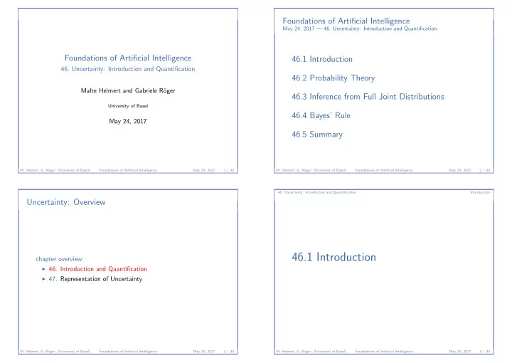
Foundations of Artificial Intelligence May 24, 2017 — 46. Uncertainty: Introduction and Quantification Foundations of Artificial Intelligence 46.1 Introduction 46. Uncertainty: Introduction and Quantification 46.2 Probability Theory Malte Helmert and Gabriele R¨ oger 46.3 Inference from Full Joint Distributions University of Basel 46.4 Bayes’ Rule May 24, 2017 46.5 Summary M. Helmert, G. R¨ oger (University of Basel) Foundations of Artificial Intelligence May 24, 2017 1 / 30 M. Helmert, G. R¨ oger (University of Basel) Foundations of Artificial Intelligence May 24, 2017 2 / 30 46. Uncertainty: Introduction and Quantification Introduction Uncertainty: Overview 46.1 Introduction chapter overview: ◮ 46. Introduction and Quantification ◮ 47. Representation of Uncertainty M. Helmert, G. R¨ oger (University of Basel) Foundations of Artificial Intelligence May 24, 2017 3 / 30 M. Helmert, G. R¨ oger (University of Basel) Foundations of Artificial Intelligence May 24, 2017 4 / 30
46. Uncertainty: Introduction and Quantification Introduction 46. Uncertainty: Introduction and Quantification Introduction Motivation Example Have to get from Aarau to Basel to attend a lecture at 9:00. Uncertainty in our knowledge of the world caused by ◮ partial observability, Different options: ◮ unreliable information (e.g. from sensors), ◮ 7:36–8:12 IR2256 to Basel ◮ nondeterminism, ◮ 7:40–7:53 S 23 to Olten, 8:05–9:29 IC 1058 to Basel ◮ laziness to collect more information, ◮ 7:40–7:57 IR 2160 to Olten, 8:05–9:29 IC 1058 to Basel ◮ . . . ◮ 8:13–8:24 RE 4760 to Olten, 8:30–8:55 IR 2310 to Basel Yet we have to act! ◮ leave by car at 8:00 and drive approx. 45 minutes ◮ . . . Option 1: Try to find solution that works in all possible worlds Option 1: � often there is no such solution Different utilities (travel time, cost, slack time, convenience, . . . ) Option 2: Quantify uncertainty (degree of belief) and and different probabilities of actually achieving the goal (traffic Option 2: maximize expected utility jams, accidents, broken trains, missed connections, . . . ). M. Helmert, G. R¨ oger (University of Basel) Foundations of Artificial Intelligence May 24, 2017 5 / 30 M. Helmert, G. R¨ oger (University of Basel) Foundations of Artificial Intelligence May 24, 2017 6 / 30 46. Uncertainty: Introduction and Quantification Introduction 46. Uncertainty: Introduction and Quantification Probability Theory Uncertainty and Logical Rules Example: diagnosing a dental patient’s toothache ◮ toothache → cavity Wrong: not all patients with toothache have a cavity. 46.2 Probability Theory ◮ toothache → cavity ∨ gumproblem ∨ abscess ∨ . . . Almost unlimited list of possible problems. ◮ cavity → pain Wrong: not all cavities cause pain. � Logic approach not suitable for domain like medical diagnosis. Instead: Use probabilities to express degree of belief, e.g. there is a Instead: 80% chance that the patient with toothache has a cavity. M. Helmert, G. R¨ oger (University of Basel) Foundations of Artificial Intelligence May 24, 2017 7 / 30 M. Helmert, G. R¨ oger (University of Basel) Foundations of Artificial Intelligence May 24, 2017 8 / 30
46. Uncertainty: Introduction and Quantification Probability Theory 46. Uncertainty: Introduction and Quantification Probability Theory Probability Model Factored Representation of Possible Worlds Sample space Ω is countable set of possible worlds Definition ◮ Possible worlds defined in terms of random variables. A probability model associates a numerical probability P ( ω ) ◮ variables Die 1 and Die 2 with domain { 1 , . . . , 6 } with each possible world such that for the values of two dice. ◮ Describe sets of possible worlds by logical formulas (called 0 ≤ P ( ω ) ≤ 1 for every ω ∈ Ω and propositions) over random variables. ◮ Die 1 = 1 � P ( ω ) = 1 . ◮ (Die 1 = 2 ∨ Die 1 = 4 ∨ Die 1 = 6) ∧ (Die 2 = 2 ∨ Die 2 = 4 ∨ Die 2 = 6) ω ∈ Ω ◮ also use informal descriptions if meaning is clear, For Ω ′ ⊆ Ω the probability of Ω ′ is defined as e.g. “both values even” � P (Ω ′ ) = P ( ω ) . ω ∈ Ω ′ M. Helmert, G. R¨ oger (University of Basel) Foundations of Artificial Intelligence May 24, 2017 9 / 30 M. Helmert, G. R¨ oger (University of Basel) Foundations of Artificial Intelligence May 24, 2017 10 / 30 46. Uncertainty: Introduction and Quantification Probability Theory 46. Uncertainty: Introduction and Quantification Probability Theory Probability Model: Example Relationships Two dice ◮ Ω = {� 1 , 1 � , . . . , � 1 , 6 � , . . . , � 6 , 1 � , . . . , � 6 , 6 �} The following rules can be derived from the definition of a probability model: ◮ P ( � x , y � ) = 1 / 36 for all x , y ∈ { 1 , . . . , 6 } (fair dice) ◮ P ( a ∨ b ) = P ( a ) + P ( b ) − P ( a ∧ b ) ◮ P ( {� 1 , 1 � , � 1 , 2 � , � 1 , 3 � , � 1 , 4 � , � 1 , 5 � , � 1 , 6 �} ) = 6 / 36 = 1 / 6 ◮ P ( ¬ a ) = 1 − P ( a ) ◮ Propositions to describe sets of possible worlds ◮ P (Die 1 = 1) = 1 / 6 ◮ P (both values even) = P ( {� 2 , 2 � , � 2 , 4 � , � 2 , 6 � , � 4 , 2 � , � 4 , 4 � , � 4 , 6 � , � 4 , 2 � , � 4 , 4 � , � 4 , 6 �} ) = 9 / 36 = 1 / 4 ◮ P (Total ≥ 11) = P ( {� 6 , 5 � , � 5 , 6 � , � 6 , 6 �} ) = 3 / 36 = 1 / 12 M. Helmert, G. R¨ oger (University of Basel) Foundations of Artificial Intelligence May 24, 2017 11 / 30 M. Helmert, G. R¨ oger (University of Basel) Foundations of Artificial Intelligence May 24, 2017 12 / 30
46. Uncertainty: Introduction and Quantification Probability Theory 46. Uncertainty: Introduction and Quantification Probability Theory Probability Distribution Joint Probability Distribution Convention: names of random variables begin with uppercase Convention: letters and names of values with lowercase letters. For multiple random variables, the joint probability distribution defines values for all possible combinations of the values. Random variable Weather with P ( Weather , Headache ) P ( Weather = sunny) = 0 . 6 headache ¬ headache P ( Weather = rain) = 0 . 1 sunny P ( sunny ∧ headache ) P ( sunny ∧ ¬ headache ) P ( Weather = cloudy) = 0 . 29 rain P ( Weather = snow) = 0 . 01 cloudy . . . Abbreviated: P ( Weather ) = � 0 . 6 , 0 . 1 , 0 . 29 , 0 . 01 � snow A probability distribution P is the vector of probabilities for the (ordered) domain of a random variable. M. Helmert, G. R¨ oger (University of Basel) Foundations of Artificial Intelligence May 24, 2017 13 / 30 M. Helmert, G. R¨ oger (University of Basel) Foundations of Artificial Intelligence May 24, 2017 14 / 30 46. Uncertainty: Introduction and Quantification Probability Theory 46. Uncertainty: Introduction and Quantification Probability Theory Conditional Probability: Intuition Conditional Probability P ( x ) denotes the unconditional or prior probability that x will Definition appear in the absence of any other information, e.g. The conditional probability for proposition a given proposition b with P ( b ) > 0 is defined as P ( cavity ) = 0 . 6 . P ( a | b ) = P ( a ∧ b ) . P ( b ) The probability of a cavity increases if we know that a patient has toothache. Example: P ( both values even | Die 2 = 4) =? P ( cavity | toothache ) = 0 . 8 Product Rule: P ( a ∧ b ) = P ( a | b ) P ( b ) � conditional probability (or posterior probability) M. Helmert, G. R¨ oger (University of Basel) Foundations of Artificial Intelligence May 24, 2017 15 / 30 M. Helmert, G. R¨ oger (University of Basel) Foundations of Artificial Intelligence May 24, 2017 16 / 30
46. Uncertainty: Introduction and Quantification Probability Theory 46. Uncertainty: Introduction and Quantification Inference from Full Joint Distributions Independence 46.3 Inference from Full Joint ◮ X and Y are independent if P ( X ∧ Y ) = P ( X ) P ( Y ). Distributions ◮ For independent variables X and Y with P ( Y ) > 0 it holds that P ( X | Y ) = P ( X ). M. Helmert, G. R¨ oger (University of Basel) Foundations of Artificial Intelligence May 24, 2017 17 / 30 M. Helmert, G. R¨ oger (University of Basel) Foundations of Artificial Intelligence May 24, 2017 18 / 30 46. Uncertainty: Introduction and Quantification Inference from Full Joint Distributions 46. Uncertainty: Introduction and Quantification Inference from Full Joint Distributions Full Joint Distribution Marginalization full joint distribution: joint distribution for all random variables. For any sets of variables Y and Z : toothache ¬ toothache � P ( Y ) = P ( Y , z ) , catch ¬ catch catch ¬ catch z ∈ Z cavity 0 . 108 0 . 012 0 . 072 0 . 008 ¬ cavity 0 . 016 0 . 064 0 . 144 0 . 576 where � z ∈ Z means to sum over all possible combinations of values of the variables in Z . Sum of entries is always 1. (Why?) P ( Cavity ) = � blackboard Sufficient for calculating the probability of any proposition. M. Helmert, G. R¨ oger (University of Basel) Foundations of Artificial Intelligence May 24, 2017 19 / 30 M. Helmert, G. R¨ oger (University of Basel) Foundations of Artificial Intelligence May 24, 2017 20 / 30
Recommend
More recommend
Explore More Topics
Stay informed with curated content and fresh updates.


