Introduction to Machine Learning ML-Basics: Data Learning goals 10 - PowerPoint PPT Presentation

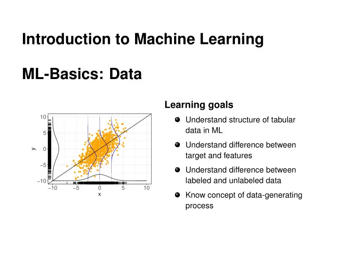
Introduction to Machine Learning ML-Basics: Data Learning goals 10 Understand structure of tabular data in ML 5 Understand difference between 0 y target and features −5 Understand difference between labeled and unlabeled data −10 −10 −5 0 5 10 Know concept of data-generating x process

IRIS DATA SET Introduced by the statistician Ronald Fisher and one of the most frequently used toy examples. Classify iris subspecies based on flower measurements. 150 iris flowers: 50 versicolor, 50 virginica, 50 setosa. Sepal length / width and petal length / width in [cm]. Source: https://rpubs.com/vidhividhi/irisdataeda Word of warning: "iris" is a small, clean, low-dimensional data set, which is very easy to classify; this is not necessarily true in the wild. � c Introduction to Machine Learning – 1 / 8

DATA IN SUPERVISED LEARNING The data we deal with in supervised learning usually consists of observations on different aspects of objects: Target : the output variable / goal of prediction Features : measurable properties that provide a concise description of the object We assume some kind of relationship between the features and the target, in a sense that the value of the target variable can be explained by a combination of the features. � c Introduction to Machine Learning – 2 / 8

ATTRIBUTE TYPES Both features and target variables may be of different data types Numerical variables can have values in R Integer variables can have values in Z Categorical variables can have values in { C 1 , ..., C g } Binary variables can have values in { 0 , 1 } For the target variable, this results in different tasks of supervised learning: regression and classification . Most learning algorithms can only deal with numerical features, although there are some exceptions (e.g. decision trees can use integers and categoricals without problems). For other feature types, we usually have to pick or create an appropriate encoding. If not stated otherwise, we assume numerical features. � c Introduction to Machine Learning – 3 / 8

OBSERVATION LABELS We call the entries of the target column labels . We distinguish two basic forms our data may come in: For labeled data we have already observed the target For unlabeled data the target labels are unknown � c Introduction to Machine Learning – 4 / 8

NOTATION FOR DATA In formal notation, the data sets we are given are of the following form: �� x ( 1 ) , y ( 1 ) � � x ( n ) , y ( n ) �� ⊂ ( X × Y ) n . D = , . . . , We call X the input space with p = dim ( X ) (for now: X ⊂ R p ), Y the output / target space, � x ( i ) , y ( i ) � ∈ X × Y the i -th observation, the tuple � T � x ( 1 ) , . . . , x ( n ) x j = the j-th feature vector. j j So we have observed n objects, described by p features. � c Introduction to Machine Learning – 5 / 8

DATA-GENERATING PROCESS We assume the observed data D to be generated by a process that can be characterized by some probability distribution P xy , defined on X × Y . We denote the random variables following this distribution by lowercase x and y . It is important to understand that the true distribution is essentially unknown to us. In a certain sense, learning (part of) its structure is what ML is all about. � c Introduction to Machine Learning – 6 / 8

DATA-GENERATING PROCESS We assume data to be drawn i.i.d. from the joint probability density function (pdf) / probability mass function (pmf) p ( x , y ) . i.i.d. stands for i ndependent and i dentically d istributed. This means: We assume that all samples are drawn from the same distribution and are mutually independent – the i -th realization does not depend on the other n − 1 ones. This is a strong yet crucial assumption that is precondition to most theory in (basic) ML. 10 5 0 y −5 −10 −10 −5 0 5 10 x � c Introduction to Machine Learning – 7 / 8

DATA-GENERATING PROCESS Remarks: With a slight abuse of notation we write random variables, e.g., x and y , in lowercase, as normal variables or function arguments. The context will make clear what is meant. Often, distributions are characterized by a parameter vector θ ∈ Θ . We then write p ( x , y | θ ) . This lecture mostly takes a frequentist perspective. Distribution parameters θ appear behind the | for improved legibility, not to imply that we condition on them in a probabilistic Bayesian sense. So, strictly speaking, p ( x | θ ) should usually be understood to mean p θ ( x ) or p ( x , θ ) or p ( x ; θ ) . On the other hand, this notation makes it very easy to switch to a Bayesian view. � c Introduction to Machine Learning – 8 / 8