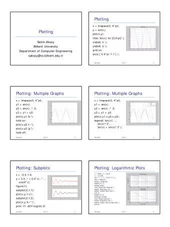
2D PLOTTING Basic Plotting plot([1,2,3,4], [1,2,1,2]) All plotting - PowerPoint PPT Presentation

2D PLOTTING

Basic Plotting plot([1,2,3,4], [1,2,1,2]) • All plotting commands have 2 similar interface: 1.8 1.6 • y-coordinates: plot(y) 1.4 • x- and y-coordinates: 1.2 1 plot(x,y) 1 1.5 2 2.5 3 3.5 4 • Most commonly used plotting scatter([1,2,3,4], [1,2,1,2]) 2 commands include the following. 1.8 1.6 • plot : Draw a line plot joining 1.4 individual data points. Typical 1.2 for plotting continuous curves 1 1 1.5 2 2.5 3 3.5 4 or long time series. scatter([1,2,3,4], [1,2,1,2]) 2 • scatter : Draw only the points. 1.5 Same as plot(x, y, ’o’) . 1 • stem : Draw points with stems. 0.5 Typical for plotting discrete 0 1 1.5 2 2.5 3 3.5 4 time series.

Plotting Many Curves • Often one wants to draw several functions into the % Define the functions to plot x = 0 : 0.01 : 2* pi ; same plot. y1 = cos (10 * x); y2 = sin (5 * x); • There are two strategies: % Plot with single command: • Enter more than one vector plot (x, y1, ’r-’, x, y2, ’b--’); to the plot (stem, scatter) % Alternatively: plot (x, y1, ’r-’); command. hold (’on’) plot (x, y2, ’b--’); • Use the hold command and hold (’off’) the previous plot is not 1 overwritten. 0.5 • In order to separate the 0 curves, we define styles as the −0.5 third argument to each plot −1 0 1 2 3 4 5 6 7 (e.g., ’b--’ )

Plot Styles • There are many di ff erent plot style strings ( help plot ):

Subplots % 6 subplots arranged in a 3x2 grid • By default, there is one plot % The last argument defines where to plot per figure. subplot (3, 2, 1); % Plot #1 plot (x, y1); title (’1st plot’); • However, one may want to subplot (3, 2, 2); % Plot #2 plot (x, y2, ’r-’); draw several axes on the same title (’2nd plot’); subplot (3, 2, 3); % Plot #3 plot, and arrange plot sizes scatter( rand (100,1), rand (100,1)); better. title (’3rd plot’); subplot (3, 2, 4); % Plot #4 [X, Fs] = audioread(’handel.ogg’); • Command subplot defines spectrogram(X, 512, 256, 256, Fs) title (’4th plot’); many axes into the same subplot (3, 2, 5); % Plot #5 scatter(y1, y2, ’k’); window. title (’5th plot’); subplot (3, 2, 6); % Plot #6 • Result of this code shown on img = imread(’ngc6543a.jpg’); imshow(img); next page. title (’6th plot’);

Subplots

Annotations • The subplots were marked plot (x, y1, ’g-’, x, y2, ’k-- with a title on top of each plot. ’) axis ([0, 2* pi , -1.5, 1.5]); • There are many other legend ({’Sine’, ’Cosine’}); xlabel (’Time’); annotation tools to add text, ylabel (’Oscillation’); title (’Two Oscillating arrows, lines, legends, etc. on Functions’); the plot: annotation(’textarrow’, [0.4, 0.47], [0.2, 0.25], ’ • title : text above plot String’, ’Minimum value’ ); • xlabel : text for x-axis grid (’on’); • ylabel : text for y-axis Two Oscillating Functions 1.5 • legend : names for curves Sine Cosine 1 • grid : grid on and o ff 0.5 • annotation : arrows, lines, Oscillation 0 text, etc. −0.5 • Note: Annotations can also be −1 Minimum value inserted interactively from −1.5 0 1 2 3 4 5 6 Time figure window.

Other Fancy Plots Multiple Decay Rates 200 1 Other 2D visualization tools include 100 0.5 Slow Decay Fast Decay the following. 0 0 −100 −0.5 • plotyy : Add two y-axes on the −200 −1 same plot. 0 0 5 5 10 10 15 15 20 20 Time ( µ sec) Logarithmic Plot • semilogx, semilogy, loglog : 5 10 Logarithmic plots. 0 10 • pie, histogram, bar : Pie −5 10 charts, etc. −10 10 −2 0 2 10 10 10 • polar, rose, compass : Angular plots. Box plot • errorbar, boxplot : Confidence 40 30 intervals. 20 10

DATA IMPORT AND EXPORT

Importing Data • Matlab has its own file format for storing data and variables. • However, not all applications produce Matlab compatible file formats. • In such cases, a low level simple data format may be required as an intermediate step (such as csv). • Matlab has several utilities for importing data from widely used formats.

Matlab Native File Format % Save the entire workspace • Matlab has its own file format >> X = [1;2;3]; that can easily store and >> save data.mat % Save all variables >> clear all % Clear everything recover the entire workspace. >> load data.mat % Load all variables >> disp (X) • The default format is binary 1 2 file, which may contain any 3 Matlab data type including % Save data into txt format. their names. % Note: The variable names are not stored, % so recovery may be difficult. • When loaded, the values get >> save data.txt -ascii their original names (this may >> type data.txt in fact be confusing). 1.0000000e+00 2.0000000e+00 • Variants of the save command 3.0000000e+00 allow saving in ascii format. % Save only variables X and Y: • However, the ascii file does >> save data.mat X Y not store variable names.

The CSV Format • The CSV format (Comma Separated Values) is one of the >> X = [1,2,3;4,5,6]; most widely used generic >> csvwrite (’data.csv’, X) % Save to CSV data container formats. >> type data.csv 1,2,3 • Commands csvread and 4,5,6 >> X2 = csvread (’data.csv’); % Load CSV csvwrite are typically enough for numeric data >> type CarPrices.csv input and output. Model;Year;Price Ford;2009;9500 • However, CSV stored from, Peugeot;2008;8000 Toyota;2011;11000 e.g., Excel may contain >> X = csvread (’CarPrices.csv’); non-numeric columns and Error using dlmread ( line 138) Mismatch between file and format string. rows. • Such more complicated files can be read by textscan .

The CSV Format with Text • textscan allows specifying % Open the file for reading: >> fid = fopen (’CarPrices.csv’, ’r’); the data types at each row. % Scan the contents. % Omit 1 line from beginning. • This is done using a format % Values are separated by ’;’ string similar to printf in C. >> C = textscan(fid, ’%s%d%d’,... >> ’HeaderLines’, 1,... • In the attached example, the >> ’Delimiter’, ’;’); format string %s%d%d states % The result is a ’cell’, % each item containing one column; that each row contains a string >> disp (C{1}) ( %s ) and two integers ( %d ) ’Ford’ ’Peugeot’ separated by ’;’ . ’Toyota’ • Other usual format specifiers >> A = horzcat(C{2:3}); % Cell to matrix >> disp (A) include 2009 9500 2008 8000 • Floating point number: %f 2011 11000 • 8-bit integer: %d8 (to save >> fclose (fid); % Close file space).

The Excel Format >> [num,txt,raw] = xlsread(’CarPrices.xlsx’) • Excel files are well num = supported. 2009 9500 2008 8000 • Basic commands: xlsread 2011 11000 and xlswrite . txt = • The xls reader returns ’Model’ ’Year’ ’Price’ three outputs: ’Ford’ ’’ ’’ ’Peugeot’ ’’ ’’ • num : A matrix with all ’Toyota’ ’’ ’’ numerical values found. • txt : A cell array with all raw = textual values found. ’Model’ ’Year’ ’Price’ ’Ford’ [2009] [ 9500] • raw : A cell array with all ’Peugeot’ [2008] [ 8000] values found. ’Toyota’ [2011] [11000]

The HDF5 Format • Hierarchical Data Format % Load example HDF5 file that comes (HDF) appears often with % with Matlab large datasets. >> info = h5info(’example.h5’) • Allows tree structured info = storage and access to the Filename: ’/matlab/demos/example.h5’ Name: ’/’ data; resembling the unix Groups: [4x1 struct] Datasets: [] directory tree. Datatypes: [] Links: [] • The example illustrates the Attributes: [2x1 struct] use of h5info command >> info .Groups(:).Name that is used for exploring /g1 the file contents. /g2 /g3 • In this case, the file /g4 contains four datasets called g1,...,g4

The HDF5 Format • The commands h5read % See subsets of dataset number 2: and h5write take care of >> info .Groups(2).Datasets.Name reading and writing the dset2.1 HDF5 files. dset2.2 % Load the latter one • The only non-trivial thing >> D = h5read(’example.h5’, ’/g2/dset2.2’) is finding the correct "path" D = inside the file. 0 0 0 • However, the file hierarchy 0.1000 0.2000 0.3000 0.2000 0.4000 0.6000 is usually described by the 0.3000 0.6000 0.9000 0.4000 0.8000 1.2000 original creator of the data.

Image, Video and Audio >> image = imread(’ngc6543a.jpg’); >> size ( image ) • Matlab is often used for ans = image and audio 650 600 3 processing. • These can be conveniently >> [audio, Fs] = audioread(’handel.mp3’); loaded to Matlab: >> size (audio) ans = • imread reads almost any image format. 73113 1 • VideoReader reads movies in all formats >> movie = VideoReader(’freqResponse.mp4’); >> videoFrames = read( movie ); that have a codec >> size (videoFrames) installed. ans = • audioread reads WAV, 900 1200 3 98 FLAC, MP3, MP4 and % Dimensions are: OGG audio formats. % height, width, color channels , frames