201ab Quantitative methods Multiple regression (b) With great - PowerPoint PPT Presentation

201ab Quantitative methods Multiple regression (b) With great illustrations from Julian Parris. E D V UL | UCSD Psychology

Multiple regression • Review • Coefficient of “partial determination” (partial R 2 , partial eta 2 ) • Nested models • Non-nested models • Polynomial regression • Multiple regression diagnostics • Partial correlations and mediation analyses E D V UL | UCSD Psychology

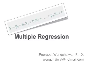
Regression Y i = β 0 + β 1 X 1 i + β 2 X 2 i + ε i 2 ) ε i ~ N (0, σ ε Coefficients: - Partial slope: dY/dX j holding other Xs constant. Multicolinearity: - Correlation among predictors. - Credit assignment is uncertain - Coefficients change; are sensitive to model and noise; have higher marginal errors. summary(lm(daughter~dad+mom)) Coefficients: Estimate Std. Error t value Pr(>|t|) (Intercept) 3.7872 4.6471 0.815 0.417082 mom 0.5210 0.1164 4.477 2.06e-05 * E D V UL | UCSD Psychology dad 0.3900 0.1078 3.617 0.000475 *

SST (SS total, also SSY) SSR[X1] SSE[X1] Variability in Y left over after factoring in X1 SSR[X1] SSE[X1,X2] SSR[X2|X1] SSR[X2] SSR[X1|X2] SSE[X1,X2] Extra sums of squares: Extra variability accounted for by taking into Variability account X1 after having considered X2. unaccounted e.g., Additional variability in daughters’ heights accounted for by taking into account for by X1 & X2 mothers’ heights having already considered fathers’ height SSR[X1,X2] SSE[X1,X2] Variability in Y accounted for by X1 & X2 e.g., Variability in daughters’ heights accounted for by mothers’ and fathers’ height E D V UL | UCSD Psychology

SST (SS total, also SSY) SSE[X1,X2] SSR[X1,X2] ! $ SS: Sum of squares for this term SS term # & d.f. of regression term: # parameters of this term df term " % F ( df term , df error ) = ! $ SSE: Sum of squared residuals SSE FULL # & df error d.f. error: n minus # parameters in full model " % SSR[X1] SSR[X2|X1] SSE[X1,X2] anova(lm(son~mom+dad)) Response: son Df Sum Sq Mean Sq F value Pr(>F) mom 1 79.523 79.523 15.3977 0.00572 ** dad 1 9.225 9.225 1.7862 0.22320 Residuals 7 36.152 5.165 SSR[X2] SSR[X1|X2] SSE[X1,X2] anova(lm(son~dad+mom)) Response: son Df Sum Sq Mean Sq F value Pr(>F) dad 1 79.595 79.595 15.4116 0.005707 ** mom 1 9.153 9.153 1.7723 0.224818 E D V UL | UCSD Psychology Residuals 7 36.152 5.165

" % SSE REDUCED − SSE FULL Extra sums of squares of full compared to reduced $ ' Extra parameters in full model p FULL − p REDUCED # & F ( p FULL − p REDUCED , n − p FULL ) = " % SSE FULL Remaining sums of squares error in full model $ ' n minus number of parameters in full model n − p FULL # & SSR[X1] (SS regression var 1) SSE[X1] anova(lm(y~x1)) Df Sum Sq Mean Sq F value Pr(>F) x1 1 517.18 517.18 64.373 2.263e-12 * Residuals 98 787.34 8.03 SSE[X1,X2,X3 SSR[X1,X2,X3] ] anova(lm(y~x1+x2+x3)) SSX[X2,X3|X1] Df Sum Sq Mean Sq F value Pr(>F) x1 1 517.18 517.18 545.73 < 2.2e-16 * x2 1 460.22 460.22 485.62 < 2.2e-16 * x3 1 236.15 236.15 249.19 < 2.2e-16 * anova( lm(y~x1) , lm(y~x1+x2+x3) ) Residuals 96 90.98 0.95 Model 1: y ~ x1 Model 2: y ~ x1 + x2 + x3 Res.Df RSS Df Sum of Sq F Pr(>F) 1 98 787.34 E D V UL | UCSD Psychology 2 96 90.98 2 696.37 367.4 < 2.2e-16 *

Significance in regression • Pairwise correlation t-test. – Is there a significant linear relationship between Y and X j ignoring other predictors? • Coefficient t-test. – Does the partial slope dY/dX j controlling for all other predictors differ significantly from zero? • Variance-partitioning F-tests. – Is the sums of squares allocated to this term (depends on order, SS type) significantly greater than chance? • Nested model comparison F-tests. – Does the larger model account for significantly more variance than the smaller model? In some special cases, these end up equivalent. E D V UL | UCSD Psychology

Multiple regression • Review • Coefficient of “partial determination” (partial R 2 , partial eta 2 ) • Nested models • Non-nested models • Polynomial regression • Multiple regression diagnostics • Partial correlations and mediation analyses E D V UL | UCSD Psychology

SST (SS total, also SSY) SSR[X1] SSE[X1] Variability in Y left over after factoring in X1 SSR[X1] SSE[X1,X2] SSR[X2|X1] SSR[X2] SSR[X1|X2] SSE[X1,X2] Extra sums of squares: Extra variability accounted for by taking into Variability account X1 after having considered X2. unaccounted e.g., Additional variability in daughters’ heights accounted for by taking into account for by X1 & X2 mothers’ heights having already considered fathers’ height SSR[X1,X2] SSE[X1,X2] Variability in Y accounted for by X1 & X2 e.g., Variability in daughters’ heights accounted for by mothers’ and fathers’ height E D V UL | UCSD Psychology

SST (SS total, also SSY) SSR[X1] (SS regression var 1) SSE[X1] (SS error) R 2 1-R 2 Proportion of variability in Y accounted for by X1 Proportion of variability e.g., Variability in daughters’ heights accounted for by mothers’ height unaccounted for by X1 “Coefficient of determination” e.g., Variability in daughters’ heights not accounted for by mothers’ height SSR[X1] SSX[X2|X1] SSE[X1,X2] SSR[X1,X2] SSE[X1,X2] R 2 Proportion of variability in Y accounted for by X1, X2 e.g., Variability in daughters’ heights accounted for by mothers’ and fathers’ height “Coefficient of multiple determination” E D V UL | UCSD Psychology

SST (SS total, also SSY) SSR[X1] (SS regression var 1) SSE[X1] (SS error) R 2 1-R 2 Proportion of variability in Y accounted for by X1 Proportion of Variability e.g., Variability in daughters’ heights accounted for by mothers’ height unaccounted for by X1 “Coefficient of determination” e.g., Variability in daughters’ heights not accounted for by mothers’ height SSR[X1] SSX[X2|X1] SSE[X1,X2] R 2Y,X2|X1 Proportion of variability previously unaccounted for by X1 that can be accounted for by X2 “Coefficient of partial determination” = SSX [ X 2 | X 1] 2 R YX 2 | X 1 SSE [ X 1] E D V UL | UCSD Psychology

Multiple regression • Review • Coefficient of “partial determination” (partial R 2 , partial eta 2 ) • Nested models • Non-nested models • Polynomial regression • Multiple regression diagnostics • Partial correlations and mediation analyses E D V UL | UCSD Psychology

• Nested Model: A smaller model that differs only by excluding some parameters of a larger model. A) height ~ mom + dad + protein + exercise + milk B) height ~ mom + dad + protein + exercise C) height ~ dad + protein + exercise D) height ~ mom + dad E) height ~ dad + protein F) height ~ mom + dad + milk G) height ~ exercise + milk + beer H) weight ~ mom + dad + protein + exercise B in A; C in A, B; D in A, B; E in A, B, C; F in A; A, G, H are not nested in others. E D V UL | UCSD Psychology

F-tests compare nested models They ask: is a bigger model better than a smaller model? height ~ mom + dad + protein + exercise + milk (nested) height ~ mom + dad + protein + exercise (nested) height ~ dad + protein + exercise (nested) height ~ protein + dad (nested) height ~ dad (nested) height ~ 1 E D V UL | UCSD Psychology 14

Extra sums of squares of full compared to reduced: Estimated by d.f. of numerator: difference in SSE. number of extra parameters in full model " % SSE REDUCED − SSE FULL $ ' p FULL − p REDUCED # & F ( p FULL − p REDUCED , n − p FULL ) = " % SSE FULL $ ' n − p FULL # & d.f. of numerator d.f. of denominator Remaining sums of squares error in full model d.f. of denominator: n minus number of parameters in full model E D V UL | UCSD Psychology

" % SSE REDUCED − SSE FULL $ ' p FULL − p REDUCED # & F ( p FULL − p REDUCED , n − p FULL ) = " % SSE FULL $ ' n − p FULL # & - Extra sums of squares of full compared to reduced model is the difference in sums of squares of error. - Degrees of freedom of the extra sums of squares is the number of parameters added. - The remaining sums of squares error from the full model is the denominator. - Degrees of freedom of error are n minus the number of parameters in full model. E D V UL | UCSD Psychology

" % SSE REDUCED − SSE FULL $ ' p FULL − p REDUCED # & F ( p FULL − p REDUCED , n − p FULL ) = " % SSE FULL $ ' n − p FULL # & SST (SS total, also SSY) SSR[X1] (SS regression var 1) SSE[X1] F = (SSR[x1] / (2-1)) / (SSE[x1] / (n-2)) • SSE reduced is just SST (a 1 parameter regression model considering only the mean of Y: B0) • SSR[X1] = SST – SSE[x1] E D V UL | UCSD Psychology

" % SSE REDUCED − SSE FULL $ ' p FULL − p REDUCED # & F ( p FULL − p REDUCED , n − p FULL ) = " % SSE FULL $ ' n − p FULL # & SSR[X1] (SS regression var 1) SSE[X1] SSE[X1,X2, SSR[X1] (SS regression var 1) SSX[X2,X3|X1] X3] F = (SSX[x2,x3|x1] / (2)) / (SSE[x1,x2,x3] / (n-4)) • SSE reduced is SSE[x1]. SSE full is SSE[x1,x2,x3] • SSX[x2,x3|x1] = SSE[x1]– SSE[x1,x2,x3] • # parameters full: 4 (b0, b1, b2, b3) • # parameters reduced: 2 (b0, b1) E D V UL | UCSD Psychology