201ab Quantitative methods L.09: Correlation, regression (2) - PowerPoint PPT Presentation

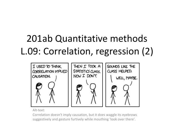
201ab Quantitative methods L.09: Correlation, regression (2) Alt-text: Correlation doesn't imply causation, but it does waggle its eyebrows suggestively and gesture furtively while mouthing 'look over there'.

Linear relationship. X and Y can be… – Independent. – Dependent, but not linearly (tricky to measure in general) – Linearly dependent (this is what we are measuring)

Ordinary, least-squares regression Least squares estimates s y ˆ β 0 = y − ˆ ˆ β 1 = r xy β 1 x s x Prediction (mean of y at each x) where the estimated line passes at each x value y i = ˆ β 0 + ˆ ˆ β 1 x i Residuals (estimated error) Deviation of real y value from line prediction ˆ ε i = y i − ˆ ( ) y i Standard deviation of residuals n 1 2 ∑ ˆ ( y i − ˆ ) σ ε = s r = y i n − 2 i = 1 The sum of squared errors: SS[e] df=n-2; we fit two parameters (B0,B1)

Regression in R Karl Pearson’s data on fathers’ and (grown) sons’ heights (England, c. 1900) fs = read.csv(url('http://vulstats.ucsd.edu/data/Pearson.csv')) f = fs$Father; s = fs$Son cor.test(f,s) t = 18.997, df = 1076, p-value < 2.2e-16 95 percent confidence interval: 0.4550726 0.5445746 sample estimates: cor 0.5011627 anova(lm(data = fs, Son~Father)) Analysis of Variance Table Response: Son Df Sum Sq Mean Sq F value Pr(>F) Father 1 2145.4 2145.35 360.9 < 2.2e-16 Residuals 1076 6396.3 5.94 summary(lm(data = fs, Son~Father)) cov(f,s) Coefficients: Estimate Std. Error t value Pr(>|t|) 3.8733 (Intercept) 33.89280 1.83289 18.49 <2e-16 Father 0.51401 0.02706 19.00 <2e-16 cor(f,s) Residual standard error: 2.438 on 1076 degrees of freedom 0.5011627 Multiple R-squared: 0.2512, Adjusted R-squared: 0.2505 F-statistic: 360.9 on 1 and 1076 DF, p-value: < 2.2e-16

Variation and randomness • In regression, ANOVA, GLM, etc. we partition variance of an outcome measure into different sources. • Our null hypotheses are that a given source contributes zero variance. • If a source contributes non-zero variance then we can use it to improve predictions of the outcome. Psych 201ab: Quantitative methods > Variation and randomness

Regression in R Karl Pearson’s data on fathers’ and (grown) sons’ heights (England, c. 1900) fs = read.csv(url('http://vulstats.ucsd.edu/data/Pearson.csv')) f = fs$Father; s = fs$Son summary(lm(data = fs, Son~Father)) Call: lm(formula = Son ~ Father, data = fs) Residuals: Min 1Q Median 3Q Max -8.8910 -1.5361 -0.0092 1.6359 8.9894 Coefficients: Estimate Std. Error t value Pr(>|t|) (Intercept) 33.89280 1.83289 18.49 <2e-16 Father 0.51401 0.02706 19.00 <2e-16 Residual standard error: 2.438 on 1076 degrees of freedom Multiple R-squared: 0.2512, Adjusted R-squared: 0.2505 F-statistic: 360.9 on 1 and 1076 DF, p-value: < 2.2e-16 anova(lm(data = fs, Son~Father)) Analysis of Variance Table Response: Son Df Sum Sq Mean Sq F value Pr(>F) Father 1 2145.4 2145.35 360.9 < 2.2e-16 Residuals 1076 6396.3 5.94 Where do all these numbers come from? What do they mean?

Sums of squares Sums of squares are handy for doing calculations by hand (which was the only option when they were developed), because you don’t have to divide or take square roots. As we have learned: they are a step along the way to getting sample variance (before we divide by the degrees of freedom). Sum of squares of X n 1 2 = “SS[X]” or “SSX” ∑ ( x i − x ) 2 s x n − 1 n ∑ ( x i − x ) 2 SS [ x ] = i = 1 i = 1 Sample variance of X Degrees of freedom for estimate of variance of X

Sums of squares So, when we are dealing with analyses of sums of squares, just keep in mind that these sums of squares are just measuring variance components (scaled by sample size). There are many things we can square and sum (and estimate the variance of) We are focused on the relationship between the last three: n ∑ ( x i − x ) 2 SS [ x ] = i = 1 SS[y] “Sum of squares of y”. n ∑ ( y i − y ) 2 SS [ y ] = Also called “SS total”, SST, SSTO, … i = 1 n SS[e] “Sum of squares of the residuals”. ∑ y i ) 2 ( y i − ˆ SS [ e ] = Also called “SS error”, SSE. i = 1 n SS[y.hat] “Sum of squares of the regression”. ∑ y i − y ) 2 SS [ ˆ ( ˆ y i ] = Also called “SS regression”, SSR, and more. i = 1

Sums of squares SS[y] “Sum of squares of y”. n ∑ ( y i − y ) 2 SS [ y ] = Also called “SS total”, SST, SSTO, … i = 1 n ∑ y i ) 2 ( y i − ˆ SS [ e ] = i = 1 n ∑ y i − y ) 2 SS [ ˆ ( ˆ y i ] = i = 1 “Sum of squares of y” “Sum of squares total” The net deviation of the ys from the mean of y

Regression in R Karl Pearson’s data on fathers’ and (grown) sons’ heights (England, c. 1900) fs = read.csv(url('http://vulstats.ucsd.edu/data/Pearson.csv')) f = fs$Father; s = fs$Son summary(lm(data = fs, Son~Father)) Call: lm(formula = Son ~ Father, data = fs) Residuals: Min 1Q Median 3Q Max -8.8910 -1.5361 -0.0092 1.6359 8.9894 Coefficients: Estimate Std. Error t value Pr(>|t|) (Intercept) 33.89280 1.83289 18.49 <2e-16 Father 0.51401 0.02706 19.00 <2e-16 Residual standard error: 2.438 on 1076 degrees of freedom Multiple R-squared: 0.2512, Adjusted R-squared: 0.2505 F-statistic: 360.9 on 1 and 1076 DF, p-value: < 2.2e-16 anova(lm(data = fs, Son~Father)) Analysis of Variance Table Response: Son Df Sum Sq Mean Sq F value Pr(>F) Father 1 2145.4 2145.35 360.9 < 2.2e-16 Residuals 1076 6396.3 5.94 Where do all these numbers come from? What do they mean?

Sums of squares Sum of squares regression. The net deviation of predicted ys from the mean of y. How much variability is captured by the regression line? n ∑ ( y i − y ) 2 SS [ y ] = i = 1 n ∑ y i ) 2 ( y i − ˆ SS [ e ] = i = 1 n SS[y.hat] “Sum of squares of the regression”. ∑ y i − y ) 2 SS [ ˆ ( ˆ y i ] = Also called “SS regression”, SSR, and more. i = 1

Regression in R Karl Pearson’s data on fathers’ and (grown) sons’ heights (England, c. 1900) fs = read.csv(url('http://vulstats.ucsd.edu/data/Pearson.csv')) f = fs$Father; s = fs$Son summary(lm(data = fs, Son~Father)) Call: lm(formula = Son ~ Father, data = fs) Residuals: Min 1Q Median 3Q Max -8.8910 -1.5361 -0.0092 1.6359 8.9894 Coefficients: Estimate Std. Error t value Pr(>|t|) (Intercept) 33.89280 1.83289 18.49 <2e-16 Father 0.51401 0.02706 19.00 <2e-16 Residual standard error: 2.438 on 1076 degrees of freedom Multiple R-squared: 0.2512, Adjusted R-squared: 0.2505 F-statistic: 360.9 on 1 and 1076 DF, p-value: < 2.2e-16 anova(lm(data = fs, Son~Father)) Analysis of Variance Table Response: Son Df Sum Sq Mean Sq F value Pr(>F) Father 1 2145.4 2145.35 360.9 < 2.2e-16 Residuals 1076 6396.3 5.94 Where do all these numbers come from? What do they mean?

Sums of squares n ∑ ( y i − y ) 2 SS [ y ] = i = 1 n SS[e] “Sum of squares of the residuals”. ∑ y i ) 2 ( y i − ˆ SS [ e ] = Also called “SS error”, SSE. i = 1 n ∑ y i − y ) 2 SS [ ˆ ( ˆ y i ] = i = 1 Sum of squares error. The net deviation of real ys from the predicted ys. How much variance is left over in the residuals?

Sums of squares n SS total ∑ ( y i − y ) 2 SS [ y ] = i = 1 n SS ∑ y i ) 2 ( y i − ˆ SS [ e ] = error i = 1 n SS ∑ y i − y ) 2 SS [ ˆ ( ˆ y i ] = regression i = 1 The deviation of y from the mean, should be equal to the deviation of the regression line from the mean, plus the deviation of y from the regression line. Similarly: SST = SSE+SSR y i − y = ( ˆ y i − y ) + ( y i − ˆ y i )

Regression in R Karl Pearson’s data on fathers’ and (grown) sons’ heights (England, c. 1900) fs = read.csv(url('http://vulstats.ucsd.edu/data/Pearson.csv')) f = fs$Father; s = fs$Son summary(lm(data = fs, Son~Father)) Call: lm(formula = Son ~ Father, data = fs) Residuals: Min 1Q Median 3Q Max -8.8910 -1.5361 -0.0092 1.6359 8.9894 Coefficients: Estimate Std. Error t value Pr(>|t|) (Intercept) 33.89280 1.83289 18.49 <2e-16 Father 0.51401 0.02706 19.00 <2e-16 Residual standard error: 2.438 on 1076 degrees of freedom Multiple R-squared: 0.2512, Adjusted R-squared: 0.2505 F-statistic: 360.9 on 1 and 1076 DF, p-value: < 2.2e-16 anova(lm(data = fs, Son~Father)) Analysis of Variance Table Response: Son Df Sum Sq Mean Sq F value Pr(>F) Father 1 2145.4 2145.35 360.9 < 2.2e-16 Residuals 1076 6396.3 5.94 Where do all these numbers come from? What do they mean?

Coefficient of determination n SS total ∑ ( y i − y ) 2 SS [ y ] = i = 1 n SS ∑ y i ) 2 ( y i − ˆ SS [ e ] = error i = 1 n SS ∑ y i − y ) 2 SS [ ˆ ( ˆ y i ] = regression i = 1 SST = SSE+SSR So, proportion of total variance accounted for by the regression: R 2 = SSR / SST Proportion left to error: 1-R 2 = SSE/SST (Yes, R 2 is just the correlation coefficient squared in this case.)