2 Two Random Variables A number of features of the two-variable - PDF document

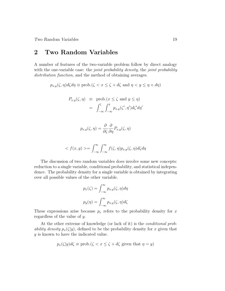
19 Two Random Variables 2 Two Random Variables A number of features of the two-variable problem follow by direct analogy with the one-variable case: the joint probability density , the joint probability distribution function , and the method of obtaining averages. p x,y ( ζ, η ) dζdη ≡ prob . ( ζ < x ≤ ζ + dζ and η < y ≤ η + dη ) P x,y ( ζ, η ) ≡ prob . ( x ≤ ζ and y ≤ η ) � ζ � η = p x,y ( ζ ′ , η ′ ) dζ ′ dη ′ −∞ −∞ ∂ ∂ p x,y ( ζ, η ) = P x,y ( ζ, η ) ∂ζ ∂η � ∞ � ∞ < f ( x, y ) > = f ( ζ, η ) p x,y ( ζ, η ) dζdη −∞ −∞ The discussion of two random variables does involve some new concepts: reduction to a single variable, conditional probability, and statistical indepen- dence. The probability density for a single variable is obtained by integrating over all possible values of the other variable. � ∞ p x ( ζ ) = p x,y ( ζ, η ) dη −∞ � ∞ p y ( η ) = p x,y ( ζ, η ) dζ −∞ These expressions arise because p x refers to the probability density for x regardless of the value of y . At the other extreme of knowledge (or lack of it) is the conditional prob- ability density p x ( ζ | y ), defined to be the probability density for x given that y is known to have the indicated value. p x ( ζ | y ) dζ ≡ prob . ( ζ < x ≤ ζ + dζ given that η = y )

20 Probability Note that in the expression p x ( ζ | y ), ζ is a variable but y is simply a pa- rameter. p x ( ζ | y ) has all the properties of a probability density function of a single random variable, ζ . The following picture may be helpful in under- standing the connection between the joint probability density p x,y ( ζ, η ) and the conditional probability density p x ( ζ | y ). ( ) = ( ( ) The specification that y is known restricts the possibilities to those lying on the line η = y in the ζ – η plane. Therefore, p x ( ζ | y ) must be proportional to p x,y ( ζ, y ): p x,y ( ζ, y ) = c p x ( ζ | y ) . The constant of proportionality, c , can be found by integrating both sides of the above equality over all ζ . � ∞ p x,y ( ζ, y ) dζ = p y ( η = y ) { reduction to a single variable } −∞ � ∞ c p x ( ζ | y ) dζ = c { normalization of p x ( ζ | y ) } −∞ � �� � 1 ⇒ c = p y ( η = y ) This result is known as Bayes’ Theorem or the fundamental law of conditional probability : p x,y ( ζ, y ) = p x ( ζ | y ) p y ( η = y )

21 Two Random Variables The result can be viewed in two ways. It can be interpreted as a way of finding the conditional density from the joint density (and the density of the conditioning event which can be recovered from the joint density): p ( x, y ) p ( x | y ) = . p ( y ) This view is illustrated in the previous figure where p ( x | y ) is exposed by ‘slicing through’ p ( x, y ). Alternatively Bayes’ theorem can be interpreted as a way of constructing the joint density from a conditional density and the probability of the conditioning variable: p ( x, y ) = p ( x | y ) p ( y ) . This is illustrated below for the two possible choices of conditioning variable. Here, as with store-bought bread, one can reassemble the loaf by stacking the individual slices side by side.

22 Probability The two random variables are said to be statistically independent (S.I.) when their joint probability density factors into a product of the densities of the two individual variables: p x,y ( ζ, η ) = p x ( ζ ) p y ( η ) if x and y are S.I. Physically, two variables are S.I. if knowledge of one gives no additional information about the other beyond that contained in its own unconditioned probability density: p ( x, y ) p ( x | y ) = = p ( x ) if x and y are S.I. p ( y ) Example: Uniform Circular Disk Given The probability of finding an event in a two dimensional space is uniform inside a circle of radius 1 and zero outside of the circle. x 2 + y 2 ≤ 1 p ( x, y ) = 1 /π x 2 + y 2 > 1 = 0 Problem Find p ( x ), p ( y ), and p ( x | y ). Are x and y S.I.? Solution √ 1 − x 2 1 √ � � 2 ∞ p ( x ) = p ( x, y ) dy = dy = 1 − x 2 | x | ≤ 1 √ 1 − x 2 π π −∞ − = 0 | x | > 1

23 Two Random Variables By symmetry, the functional form for p ( y ) will be identical. 2 � p ( y ) = 1 − y 2 | y | ≤ 1 π = 0 | y | > 1 It is apparent that the product of p ( x ) and p ( y ) does not equal p ( x, y ), so the random variables x and y are not S.I. The conditional probability is found from Bayes’ theorem. { when x 2 − y 2 } p ( x, y ) (1 /π ) ≤ 1 (2 /π ) √ 1 − y p ( x y | ) = = { when y 2 ≤ 1 } p ( y ) 2 1 � 2 √ 1 − y 2 = | x | ≤ 1 − y 2 = 0 elsewhere It is not surprising that p ( x | y ) is a constant when one considers the following interpretation.

24 Probability . . . . . . . . . . . . . . . . . . . . . . . . . . . . . . . . . . . . . Example: Derivation of the Poisson Density Given Events occurring at random alone a line X are governed by the following two conditions: • In the limit ∆ X → 0 the probability that one and only one event occurs between X and X + ∆ X is given by r ∆ X , where r is a given constant independent of X . • The probability of an event occurring in some interval ∆ X is statisti- cally independent of events in all other portions of the line. Problem a) Find the probability p ( n = 0; L ) that no events occur in a region of length L . Proceed by dividing L into an infinite number of S.I. intervals and calculate the joint probability that none of the intervals contains an event. b) Obtain the differential equation d p ( n ; L ) + rp ( n ; L ) = rp ( n − 1; L ) dL as a recursion relation governing the p(n;L).

25 Two Random Variables c) Show that the Poisson density 1 ( rL ) n e − rL p ( n ; L ) = n ! is a solution of the equation. Is it unique? Solution a) To find p ( n = 0; L ) divide L into intervals each of length dL : Consider dL so short that p (0) >> p (1) >> p ( n > 1) in dL . But the probabilities must sum to unity, p (0) + p (1) + p (2) + · · · = 1, so one can find an approximation to p (0) which will be valid in the limit of small dL . p (0) ≈ 1 − p (1) = 1 − r ( dL ) The probability of an event in any sub-interval is S.I. of the events in every other sub-interval, so m = L/dL � p ( n = 0; L ) = (1 − r ( dL )) m =1 � ln p ( n = 0; L ) = ln(1 − r ( dL )) m m = L/dL � ln p ( n = 0; L ) ≈ − r ( dL ) m =1 � L � = − r ( dL ) = − rL dL e − rL p ( n = 0; L ) =

� 26 Probability ∞ p ( n = 0; L ) dL = 1 since p ( n = 0; L ) is not a probability density � Note that 0 for L , rather it is one element of a discrete probability density for n which depends on L as a parameter. b) Now consider the span X = 0 to X = L +∆ L to be composed of the finite length L and an infinitesimal increment ∆ L . The two intervals are S.I. so one may decompose p ( n ; L + ∆ L ) in terms of two mutually exclusive events. p ( n ; L + ∆ L ) = p ( n ; L ) p (0; ∆ L ) + p ( n − 1; L ) p (1; ∆ L ) = p ( n ; L )(1 − r ∆ L ) + p ( n − 1; L )( r ∆ L ) Rearranging p ( n ; L + ∆ L ) − p ( n ; L ) = rp ( n − 1; L ) − rp ( n ; L ) ∆ L Passing to the limit ∆ L → 0 gives d p ( n ; L ) = rp ( n − 1; L ) − rp ( n ; L ) dL

� 27 Two Random Variables c) To show that the Poisson density satisfies this equation, take its derivative with respect to L and compare the result with the above expression. 1 ( rL ) n e − rL p ( n ; L ) = n ! d n 1 ( rL ) n − 1 e − rL − r ( rL ) n e − rL p ( n ; L ) = r dL n ! n ! 1 1 ( rL ) n − 1 e − rL ( rL ) n e − rL = r − r ( n − 1)! n ! = rp ( n − 1; L ) − rp ( n ; L ) This solution is unique when the differential recursion relation is supple- mented by the boundary conditions p (0; L ) = e − rL p ( n ; 0) = 0 n = 0 . . . . . . . . . . . . . . . . . . . . . . . . . . . . . . . . . . . . . . Extended Example: Jointly Gaussian Random Variables Introduction The purpose of this example is to examine a particular joint probability density and the information that can be extracted from it. We will focus our attention on a physical example that might be encountered in the laboratory. However, the origin of the effect is not of concern to us now. We are interested instead in understanding and manipulating a given probability density. The System Consider an electronic circuit with all sources (power supplies and signal inputs) turned off. If one looks at a given pair of terminals with an oscilloscope, the voltage appears to be zero at low gain, but at high gain there will be a fluctuating random voltage that might look as follows: