1 Principal Components Analysis (PCA) Review of basic setup: N - PDF document

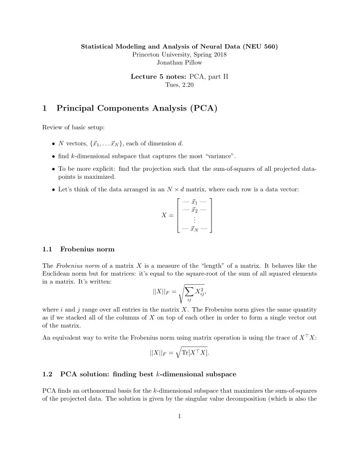
Statistical Modeling and Analysis of Neural Data (NEU 560) Princeton University, Spring 2018 Jonathan Pillow Lecture 5 notes: PCA, part II Tues, 2.20 1 Principal Components Analysis (PCA) Review of basic setup: • N vectors, { � x 1 , . . . � x N } , each of dimension d . • find k -dimensional subspace that captures the most “variance”. • To be more explicit: find the projection such that the sum-of-squares of all projected data- points is maximized. • Let’s think of the data arranged in an N × d matrix, where each row is a data vector:   — � x 1 — — � x 2 —   X =  .  .   .   — � x N — 1.1 Frobenius norm The Frobenius norm of a matrix X is a measure of the “length” of a matrix. It behaves like the Euclidean norm but for matrices: it’s equal to the square-root of the sum of all squared elements in a matrix. It’s written: �� X 2 || X || F = ij , ij where i and j range over all entries in the matrix X . The Frobenius norm gives the same quantity as if we stacked all of the columns of X on top of each other in order to form a single vector out of the matrix. An equivalent way to write the Frobenius norm using matrix operation is using the trace of X ⊤ X : � Tr[ X ⊤ X ] . || X || F = 1.2 PCA solution: finding best k -dimensional subspace PCA finds an orthonormal basis for the k -dimensional subspace that maximizes the sum-of-squares of the projected data. The solution is given by the singular value decomposition (which is also the 1

eigenvector decomposition) of X ⊤ X : ( X ⊤ X ) = USU ⊤ , The first k columns of U are the first k principal components: { � u k } . u 1 , � u 2 , . . . , � The singular values correspond to the sum-of-squares of the data vectors projected into the corre- sponding principal component: N � x i ) 2 s j = ( � u j · � i =1 1.3 Fraction of variance The squared Frobenius norm of X is (surprisingly!) equal to the sum of the singular values: N d x i || 2 = � � || X || 2 F = || � s j i =1 j =1 The fraction of the total variance accounted for by the first k principal components is therefore given by: s 1 + · · · + s k . s 1 + · · · + s k + · · · + s d 1.4 Fitting an ellipse to your data PCA is equivalent to fitting an ellipse to your data: the eigenvectors � u i give the dominant axes of the ellipse, while the s i gives the elongation of the ellipse along each axis, and is equal sum of squared projections (what we’ve been calling “variability” above) of the data along that axis. 1.5 Zero-centering So far we’ve assumed we wanted to maximize the sum of squared projections of the vectors { � x i } onto some subspace, which is equivalent to using an ellipse centered at the origin to describe the data. In most applications, we want to consider an ellipse centered on the data , and find principal components that describe the spread of the datapoints relative to the mean. To “center” the dataset at zero, we can simply subtract off the mean from each data vector. The mean is given by x = 1 � ¯ � x i N . 2

Then the zero-centered data matrix can be formed as by placing � z i = � x i − ¯ x on each row:   — � z 1 — . . Z =   .   — — � z N Then by taking the SVD of ( Z ⊤ Z ) we will be obtaining principal components of the centered data. Note: this the standard definition of PCA! It is uncommon to do PCA on uncentered data. 1.6 Python implementation In python, we can achieve zero-centering (and division by N ) with the function np.cov . That is, np.cov(X) will return 1 N ( Z ⊤ Z ) , 2 Derivation for PCA In the lectures on PCA we showed that if we restricted ourselves to considering eigenvectors of the X ⊤ X , then the eigenvector with largest eigenvalue captured the largest projected-sum-of-squares of the vectors in X . But we didn’t show that eigenvectors themselves correspond to optimal solution. To recap briefly, we want to find the maximum of v ⊤ C� � v, where C = X ⊤ X is the (scaled) covariance of zero-centered data vectors { � x i } , subject to the v ⊤ � constraint that � v is a unit vector ( � v = 1). We can solve this kind of optimization problem using the method of Lagrange multipliers. The basic idea is that we minimize a function that is our original function plus a lagrange multiplier λ times an expression that is zero when our constraint is satisfied. For this problem we can define the Lagrangian: v ⊤ C� v ⊤ � L = � v + λ ( � v − 1) . (1) We will want solutions for which ∂ v L = 0 (2) ∂� ∂ ∂λ L = 0 . (3) Note that the second of these is satisfied if and only if � v is a unit vector (which is reassuring). The first equation gives us: ∂ v L = ∂ v ⊤ � v + λ ( � v − 1) = 2 C� v − 2 λ� = 0 , (4) v � vC� v ∂� ∂� 3

which implies C� v = − λ� v. (5) What is this? It’s the eigenvector equation! This implies that the derivative of the Lagrangian is zero when � v is an eigenvector of C . So this establishes, combined with the argument from last week, that the unit vector that captures the greatest squared projection of the raw data is the top eigenvector of C . 2.1 Objective functions for PCA Formally, we can write the principal components as the columns of a d × k matrix B that maximizes the Frobenious norm of the data projected onto B : ˆ || XB || 2 B pca = arg max F B such that B ⊤ B = I . An equivalent definition is ˆ B || X − XBB ⊤ || 2 B pca = arg min F such that B ⊤ B = I . This objective function says that the principal components define an or- thonormal basis such that the distance between the original data and the data projected onto that subspace is minimal. It shouldn’t take to much effort to see that that the rows of XBB ⊤ correspond to the rows of X reconstructed in the basis defined by columns of B . 4