1 Principal Components Analysis (PCA) Suppose someone hands you a - PDF document

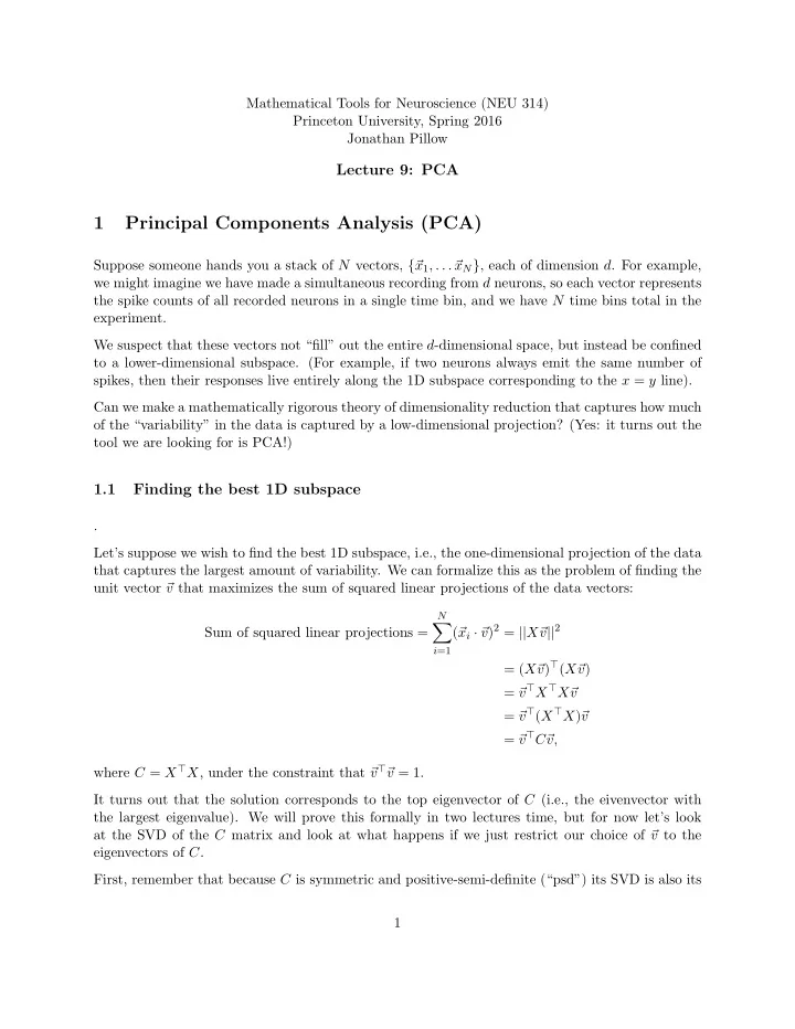
Mathematical Tools for Neuroscience (NEU 314) Princeton University, Spring 2016 Jonathan Pillow Lecture 9: PCA 1 Principal Components Analysis (PCA) Suppose someone hands you a stack of N vectors, { � x 1 , . . . � x N } , each of dimension d . For example, we might imagine we have made a simultaneous recording from d neurons, so each vector represents the spike counts of all recorded neurons in a single time bin, and we have N time bins total in the experiment. We suspect that these vectors not “fill” out the entire d -dimensional space, but instead be confined to a lower-dimensional subspace. (For example, if two neurons always emit the same number of spikes, then their responses live entirely along the 1D subspace corresponding to the x = y line). Can we make a mathematically rigorous theory of dimensionality reduction that captures how much of the “variability” in the data is captured by a low-dimensional projection? (Yes: it turns out the tool we are looking for is PCA!) 1.1 Finding the best 1D subspace . Let’s suppose we wish to find the best 1D subspace, i.e., the one-dimensional projection of the data that captures the largest amount of variability. We can formalize this as the problem of finding the unit vector � v that maximizes the sum of squared linear projections of the data vectors: N v ) 2 = || X� � v || 2 Sum of squared linear projections = ( � x i · � i =1 v ) ⊤ ( X� = ( X� v ) v ⊤ X ⊤ X� = � v v ⊤ ( X ⊤ X ) � = � v v ⊤ C� = � v, where C = X ⊤ X , under the constraint that � v ⊤ � v = 1. It turns out that the solution corresponds to the top eigenvector of C (i.e., the eivenvector with the largest eigenvalue). We will prove this formally in two lectures time, but for now let’s look at the SVD of the C matrix and look at what happens if we just restrict our choice of � v to the eigenvectors of C . First, remember that because C is symmetric and positive-semi-definite (“psd”) its SVD is also its 1

eigenvector decomposition: C = USU ⊤ , where the columns of U are the eigenvectors and diagonal entries of S are eigenvalues. Now let’s consider what happens if we set � v = � u j , i.e., the j ’th eigenvector of C . Because U is an orthogonal matrix (i.e., its columns for an orthonormal basis), then U ⊤ � u j will be a vector of zeros with a 1 in the j ’th component. We have u ⊤ u ⊤ j ( USU ⊤ ) � � j C� u j = � u j u j U ) S ( U ⊤ � = ( � u j )     s 1 0 . ... .     .     � �     = 0 · · · 1 · · · 0 1 s j     .  ...    .     .     s d 0 = s j So: plugging in the j ’th eigenvector of C gives us out s j as the sum of squared projections. Since we want to maximize this quantity (i.e., find the linear projection that maximizes it), we should clearly choose the eigenvector with largest eigenvalue, which (since SVD orders them from greatest to smallest) corresponds to the solution � v = � u 1 . This vector (the “dominant” eigenvector of C) is the first principle component (sometimes called the “first PC” for short). 1.2 Finding best k -dimensional subspace . The above solution to the more general case of finding the k -dimensional subspace. Since the eigenvectors of C are orthogonal, the variability preserved by each projection is independent of the variability preserved by the other eigenvectors. Thus, a basis for the k -dimensional subspace that preserves the greatest variability is given by the first k eigenvectors of C : � � First k PCs = � u 1 , . . . , � u k The total “variability” captured by these principal components is given by: N N u 1 ) 2 + · · · + u k ) 2 = || X� u 1 || 2 + · · · + || X� � � u k || 2 ( � x i · � ( � x i · � i =1 i =1 = s 1 + · · · + s k 2

The variability of the entire x set of vectors is equal to N x i || 2 = s 1 + · · · + s d . � || � i =1 (Verify for yourself that this is true!) The fraction of the variability captured by the first k principal components is therefore given by s 1 + · · · + s k . s 1 + · · · + s k + · · · + s d subsectionZero-centered data PCA is tantamount to fitting an ellipse to your data: the eigenvectors � u i give the dominant axes of the ellipse, while the s i gives the elongation of the ellipse along each axis, and is equal sum of squared projections (what we’ve been calling “variability” above) of the data along that axis. So far we’ve assumed we wanted to maximize the sum of squared projections of the vector { � x j } , which is equivalent to fitting an ellipse centered at zero and examining major axes of that ellipse. In many settings, however, we would prefer to examine the dimensionality of the data by considering an ellipse centered on the centroid (the arithmetic mean) of the data. We can achieve this by simply subtracting off the mean of the data from each data vector. The mean is given by x = 1 � ¯ � x i N . We can call define the centered data matrix as     — � x 1 — — x ¯ — . . ˜ . . X =  −  ,     . .   — — — ¯ — x N � x that is, a matrix in which we subtract off the mean vector ¯ x from each row. Then by taking the X ⊤ ˜ eigenvectors of ( ˜ X ) we will be obtaining principal components of the centered data. Note: this is the standard definition of PCA! It is uncommon to do PCA on uncentered data. 1.3 Notes on Matlab implementation • We can center the data simply in matlab (i.e., without using a for loop) via the command Xctr = X - repmat(mean(X),N,1); . • PCA is obtained by two additional lines: [U,S] = svd(Xctr'*Xctr); PCs_1toK = U(:,1:k); 3

• An even simpler method is to use cov , which computes the sample covariance matrix of the X ⊤ ˜ data. This centers the data and divides the ˜ X matrix by N (or N − 1, which is the default in Matlab). The resulting code for PCA is simply: [U,S] = svd(cov(X)); PCs_1toK = U(:,1:k); • We can get the variance captured by each PC in a single vector using: s_vec = diag(S(1:k,1:k)); 4