Lecture: Face Recognition and Feature Reduction Juan Carlos Niebles - PowerPoint PPT Presentation
Dimensionality Reduction Lecture: Face Recognition and Feature Reduction Juan Carlos Niebles and Ranjay Krishna Stanford Vision and Learning Lab 31-Oct-2019 1 St Stanfor ord University CS 131 Roadmap Dimensionality Reduction Pixels
Dimensionality Reduction Lecture: Face Recognition and Feature Reduction Juan Carlos Niebles and Ranjay Krishna Stanford Vision and Learning Lab 31-Oct-2019 1 St Stanfor ord University
CS 131 Roadmap Dimensionality Reduction Pixels Segments Images Videos Web Recognition Neural networks Convolutions Resizing Motion Detection Convolutional Edges Segmentation Tracking Machine learning neural networks Descriptors Clustering 31-Oct-2019 2 St Stanfor ord University
Recap - Curse of dimensionality • Assume 5000 points uniformly distributed in the unit hypercube and we want to apply 5-NN. Suppose our query point is at the origin. – In 1-dimension, we must go a distance of 5/5000=0.001 on the average to capture 5 Dimensionality Reduction nearest neighbors. – In 2 dimensions, we must go to get a square that contains 0.001 of the volume. – In d dimensions, we must go 0.001 1/ d ( ) 0.001 31-Oct-2019 3 Stanfor St ord University
What we will learn today • Singular value decomposition Dimensionality Reduction • Principal Component Analysis (PCA) • Image compression 31-Oct-2019 4 St Stanfor ord University
What we will learn today • Singular value decomposition Dimensionality Reduction • Principal Component Analysis (PCA) • Image compression 31-Oct-2019 5 St Stanfor ord University
Singular Value Decomposition (SVD) Dimensionality Reduction • There are several computer algorithms that can “factorize” a matrix, representing it as the product of some other matrices • The most useful of these is the Singular Value Decomposition. • Represents any matrix A as a product of three matrices: UΣV T • Python command: – [U,S,V]= numpy.linalg.svd(A ) 31-Oct-2019 6 St Stanfor ord University
Singular Value Decomposition (SVD) Dimensionality Reduction UΣV T = A • Where U and V are rotation matrices, and Σ is a scaling matrix. For example: 31-Oct-2019 7 St Stanfor ord University
Singular Value Decomposition (SVD) • Beyond 2x2 matrices: – In general, if A is m x n , then U will be m x m , Σ will be m x n , and V T will be n x n . Dimensionality Reduction – (Note the dimensions work out to produce m x n after multiplication) 31-Oct-2019 8 St Stanfor ord University
Singular Value Decomposition (SVD) • U and V are always rotation matrices. Dimensionality Reduction – Geometric rotation may not be an applicable concept, depending on the matrix. So we call them “unitary” matrices – each column is a unit vector. • Σ is a diagonal matrix – The number of nonzero entries = rank of A – The algorithm always sorts the entries high to low 31-Oct-2019 9 St Stanfor ord University
SVD Applications • We’ve discussed SVD in terms of geometric transformation matrices Dimensionality Reduction • But SVD of an image matrix can also be very useful • To understand this, we’ll look at a less geometric interpretation of what SVD is doing 31-Oct-2019 10 St Stanfor ord University
SVD Applications Dimensionality Reduction • Look at how the multiplication works out, left to right: • Column 1 of U gets scaled by the first value from Σ . 31-Oct-2019 • The resulting vector gets scaled by row 1 of V T to produce a contribution to the columns of A 11 St Stanfor ord University
SVD Applications Dimensionality Reduction + = 31-Oct-2019 • Each product of ( column i of U ) · ( value i from Σ ) · ( row i of V T ) produces a component of the final A . 12 St Stanfor ord University
SVD Applications Dimensionality Reduction • We’re building A as a linear combination of the columns of U • Using all columns of U , we’ll rebuild the original matrix perfectly 31-Oct-2019 • But, in real-world data, often we can just use the first few columns of U and we’ll get something close (e.g. the first A partial , above) 13 St Stanfor ord University
SVD Applications Dimensionality Reduction • We can call those first few columns of U the Principal Components of the data 31-Oct-2019 • They show the major patterns that can be added to produce the columns of the original matrix • The rows of V T show how the principal components are mixed to produce the columns of the matrix 14 St Stanfor ord University
SVD Applications Dimensionality Reduction We can look at Σ while the second to see that the column has a much first column has a smaller effect in this large effect 31-Oct-2019 example 15 St Stanfor ord University
SVD Applications Dimensionality Reduction • For this image, using only the first 10 of 300 principal components produces a recognizable 31-Oct-2019 reconstruction • So, SVD can be used for image compression 16 St Stanfor ord University
SVD for symmetric matrices • If A is a symmetric matrix, it can be decomposed as the following: Dimensionality Reduction • Compared to a traditional SVD decomposition, U = V T and is an orthogonal matrix. 31-Oct-2019 17 St Stanfor ord University
Principal Component Analysis Dimensionality Reduction • Remember, columns of U are the Principal Components of the data: the major patterns that can be added to produce the columns of the original matrix • One use of this is to construct a matrix where each column is a separate data sample • Run SVD on that matrix, and look at the first few columns of U to see 31-Oct-2019 patterns that are common among the columns • This is called Principal Component Analysis (or PCA) of the data samples 18 St Stanfor ord University
Principal Component Analysis Dimensionality Reduction • Often, raw data samples have a lot of redundancy and patterns • PCA can allow you to represent data samples as weights on the principal components, rather than using the original raw form of the data • By representing each sample as just those weights, you can represent just the “meat” of what’s different between samples. 31-Oct-2019 • This minimal representation makes machine learning and other algorithms much more efficient 19 St Stanfor ord University
How is SVD computed? • For this class: tell PYTHON to do it. Use the result. Dimensionality Reduction • But, if you’re interested, one computer algorithm to do it makes use of Eigenvectors! 31-Oct-2019 20 St Stanfor ord University
Eigenvector definition • Suppose we have a square matrix A . We can solve for vector x and scalar λ such Dimensionality Reduction that Ax= λx • In other words, find vectors where, if we transform them with A , the only effect is to scale them with no change in direction. • These vectors are called eigenvectors (German for “self vector” of the matrix), and the scaling factors λ are called eigenvalues • An m x m matrix will have ≤ m eigenvectors where λ is nonzero 31-Oct-2019 21 St Stanfor ord University
Finding eigenvectors • Computers can find an x such that Ax= λx using this iterative algorithm: Dimensionality Reduction – X = random unit vector – while(x hasn’t converged) • X = Ax • normalize x • x will quickly converge to an eigenvector 31-Oct-2019 • Some simple modifications will let this algorithm find all eigenvectors 22 St Stanfor ord University
Finding SVD Dimensionality Reduction • Eigenvectors are for square matrices, but SVD is for all matrices • To do svd(A), computers can do this: – Take eigenvectors of AA T (matrix is always square). • These eigenvectors are the columns of U . • Square root of eigen values are the singular values (the entries of Σ ). – Take eigenvectors of A T A (matrix is always square). • These eigenvectors are columns of V (or rows of V T ) 31-Oct-2019 23 St Stanfor ord University
Finding SVD Dimensionality Reduction • Moral of the story: SVD is fast, even for large matrices • It’s useful for a lot of stuff • There are also other algorithms to compute SVD or part of the SVD – Python’s np.linalg.svd() command has options to efficiently compute only what you need, if performance becomes an issue 31-Oct-2019 A detailed geometric explanation of SVD is here: http://www.ams.org/samplings/feature-column/fcarc-svd 24 St Stanfor ord University
What we will learn today • Introduction to face recognition Dimensionality Reduction • Principal Component Analysis (PCA) • Image compression 31-Oct-2019 25 St Stanfor ord University
Covariance • Variance and Covariance are a measure of the “spread” of a set of points around Dimensionality Reduction their center of mass (mean) • Variance – measure of the deviation from the mean for points in one dimension e.g. heights • Covariance as a measure of how much each of the dimensions vary from the mean with respect to each other. • Covariance is measured between 2 dimensions to see if there is a relationship between the 2 dimensions e.g. number of hours studied & marks obtained. 31-Oct-2019 • The covariance between one dimension and itself is the variance 26 St Stanfor ord University
Covariance Dimensionality Reduction • So, if you had a 3-dimensional data set (x,y,z), then you could measure the 31-Oct-2019 covariance between the x and y dimensions, the y and z dimensions, and the x and z dimensions. Measuring the covariance between x and x , or y and y , or z and z would give you the variance of the x , y and z dimensions respectively 27 St Stanfor ord University
Recommend
More recommend
Explore More Topics
Stay informed with curated content and fresh updates.

