1 Linearity and Linear Systems Linear system is a kind of mapping f - PDF document

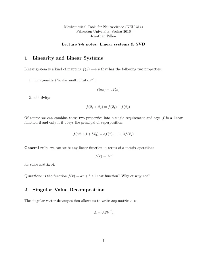
Mathematical Tools for Neuroscience (NEU 314) Princeton University, Spring 2016 Jonathan Pillow Lecture 7-8 notes: Linear systems & SVD 1 Linearity and Linear Systems Linear system is a kind of mapping f ( � x ) − → � y that has the following two properties: 1. homogeneity (“scalar multiplication”): f ( ax ) = af ( x ) 2. additivity: f ( � x 1 + � x 2 ) = f ( � x 1 ) + f ( � x 2 ) Of course we can combine these two properties into a single requirement and say: f is a linear function if and only if it obeys the principal of superposition: f ( a� x + 1 + b� x 2 ) = af ( � x ) + 1 + bf ( � x 2 ) . General rule : we can write any linear function in terms of a matrix operation: f ( � x ) = A� x for some matrix A . Question : is the function f ( x ) = ax + b a linear function? Why or why not? 2 Singular Value Decomposition The singular vector decomposition allows us to write any matrix A as A = USV ⊤ , 1

where U and V are orthogonal matrices (square matrices whose columns form an orthonormal basis), and S is a diagonal matrix (a matrix whose only non-zero entries lie along the diagonal):   s 1 s 2   S =   ...     s n The columns of U and V are called the left singular vectors and right singular vectors , respectively. The diagonal entires { s i } are called singular values . The singular values are always ≥ 0. The SVD tells us that we can think of the action of A upon any vector � x in terms of three steps: 1. rotation (multiplication by V ⊤ , which doesn’t change length of � x ). 2. stretching along the cardinal axes (where the i ′ th component is stretched by s i ). 3. another rotation (multipication by U ). 3 Applications of SVD 3.1 Inverses The SVD makes it easy to compute (and understand) the inverse of a matrix. We exploit the fact that U and V are orthogonal, meaning their transposes are their inverses, i.e., U ⊤ U = UU ⊤ = I and V ⊤ V = V V ⊤ = I . The inverse of A (if it exists) can be determined easilly from the SVD, namely: A − 1 = V S − 1 U T , where 1   s 1 1 S − 1 =   s 2   ...     1 s n The logic is that we can find the inverse mapping by undoing each of the three operations we did when multiplying A : first, undo the last rotation by multiplying by U ⊤ ; second, un-stretch by multiplying by 1 /s i along each axis, third, un-rotate by multiplying by V . 2

Another way to see that this definition of the inverse is correct is via: A − 1 A = ( V S − 1 U ⊤ )( USV ⊤ ) = V S − 1 ( U ⊤ U ) SV ⊤ = V ( S − 1 S ) V ⊤ = V V ⊤ = I We can do a similar analysis of AA − 1 . 3.2 Pseudo-inverse The SVD also makes it easy to see when the inverse of a matrix doesn’t exist. Namely, if any of the singular values s i = 0, then the S − 1 doesn’t exist, because the corresponding diagonal entry would be 1 /s i = 1 / 0. In other words, if a matrix A has any zero singular values (let’s say s j = 0), then multiplying by A effectively destroys information because it takes the component of the vector along the right singular vector � v j and multiplies it by zero. We can’t recover this information, so there’s no way to “invert” the mapping A� x to recover the original � x that came in. The best we can do is to recover the components of � x that weren’t destroyed via multiplication with zero. The matrix that recovers all recoverable information is called the pseudo-inverse , and is often denoted A † . We can obtain the pseudoinverse from the SVD by inverting all singular values that are non-zero, and leaving all zero singular values at zero. Suppose we have an n × n matrix A , which has only k non-zero singular values. Then the S matrix obtained from SVD will be   s 1 ...       s k   S = .   0     ...     0 The pseudoinverse of A can then be written similarly to the inverse: A † = V S † U ⊤ , 3

where 1   s 1 ...      1  S † =   s k .   0     ...     0 • rank : It is easy to show that the rank of A is k (since there columns of A can all be formed as a linear combination of the first k columns of U ). • singular matrix : a matrix that is not full rank (and therefore does not have an inverse) is called singular . • row space and null space The first k columns of V (i.e., the first k rows of V ⊤ will provide an orthonormal basis for the of A . The remaining n − k columns of V will provide an orthonormal basis for the null space of A . 3.3 Condition number In practical situations, a matrix may have singular values that are not exactly equal to zero, but are so close to zero that it is not possible to accurately compute them. In such cases, the matrix is what we call ill-conditioned , because dividing by the singular values (1 /s i ) for singular values s i that are arbitrarily close to zero will result in numerical errors. Such matrices are theoretically but not practically invertible. (If you try to invert such a matrix, matlab will produce a warning: “Matrix is close to singular”). The degree to which ill-conditioning prevents a matrix from being inverted accurately depends on the ratio of its largest to smallest singular value, a quantity known as the condition number: condition number = s 1 . s n The larger the condition number, the more practically non-invertible it is. In matlab condition numbers greater than ≈ 10 14 indicate the matrix cannot be stably inverted. You can computed the condition number from the SVD, or using the built-in matlab command cond . 3.4 SVD of non-square matrix If A m × n is a non-square matrix, then U is m × m and V is n × n , and S m × n is non-square (and therefore has only min(m , n) non-zero singular values. 4

3.5 Relationship between SVD and eigenvector decomposition Definition : Recall that an eigenvector of a square matrix A is defined as a vector satisfying the equation A� x = λ� x, and λ is the corresponding eigenvalue . In other words, an eigenvector of A is any vector that, when multiplied by A , comes back as itself scaled by λ . Spectral theorem : If a matrix A is symmetric and positive semi-definite (i.e., its eigenvalues are all ≥ 0), then the SVD also an eigendecomposition, that is, a decomposition in terms of an orthonormal basis of eigenvectors: A = USU ⊤ , where the columns of U are eigenvectors and the diagonal entries { s i } of S are the eigenvalues. (Note that U = V , meaning the left and right singular vectors are identical, and equal to the eigenvectors.) 5