Workshop 7: (Generalized) Linear models Murray Logan 19 Jul 2017 - - PowerPoint PPT Presentation

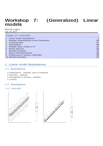
Workshop 7: (Generalized) Linear models

Murray Logan 19 Jul 2017

Section 1 Linear model Assumptions

Assumptions

• Independence - unbiased, scale of

treatment

• Normality - residuals
• Homogeneity of variance - residuals
• Linearity

Assumptions

N

• r

m a l i t y

• y
• y

Assumptions

H

• m
• g

e n e i t y

• f

v a r i a n c e

• ●
• ●
• ●
• y

X Y

• ● ●
• ●
• x

y

• ●
• res

Predicted x Residuals

• ●
• ●
• ●
• y

X Y

• x

y

• res

Predicted x Residuals

Assumptions

L i n e a r i t y

Trendline

• 5

10 15 20 25 30 10 20 30 40 50 60

• 5

10 15 20 25 30 0.0 0.5 1.0 1.5 2.0 2.5

Assumptions

L i n e a r i t y

Loess (lowess) smoother

• 5

10 15 20 25 30 10 20 30 40 50 60

• 2.0

2.5

Assumptions

L i n e a r i t y

Spline smoother

• 5

10 15 20 25 30 10 20 30 40 50 60

• 5

10 15 20 25 30 0.0 0.5 1.0 1.5 2.0 2.5

Assumptions

yi = β0 + β1 × xi + εi

ϵi ∼ N(0, σ2)

Assumptions

yi = β0 + β1 × xi + εi

ϵi ∼ N(0, σ2)

The linear predictor

y = β0 + β1x Y X 3 2.5 1 6 2 5.5 3 9 4 8.6 5 12 6

3.0 = β0 × 1 + β1 × 0 2.5 = β0 × 1 + β1 × 1 6.0 = β × 1 + β × 2

Response values Model matrix Parameter vector

Linear models in R

> lm(formula, data= DATAFRAME)

Model R formula Description yi = β0 + β1xi

y~1+x y~x

Full model yi = β0

y~1

Null model yi = β1

y~-1+x

Through origin

> lm(Y~X, data= DATA) Call: lm(formula = Y ~ X, data = DATA) Coefficients: (Intercept) X 2.136 1.507

Linear models in R

> Xmat = model.matrix(~X, data=DATA) > Xmat (Intercept) X 1 1 0 2 1 1 3 1 2 4 1 3 5 1 4 6 1 5 7 1 6 attr(,"assign") [1] 0 1 > lm.fit(Xmat,DATA$Y) $coefficients (Intercept) X 2.135714 1.507143 $residuals [1] 0.8642857 -1.1428571 0.8500000 -1.1571429 0.8357143 -1.0714286 0.8214286 $effects (Intercept) X

• 17.6131444

7.9750504 0.6507186 -1.5697499 0.2097817 -1.9106868 -0.2311552 $rank [1] 2 $fitted.values [1] 2.135714 3.642857 5.150000 6.657143 8.164286 9.671429 11.178571 $assign [1] 0 1 $qr $qr (Intercept) X 1

• 2.6457513 -7.93725393

2 0.3779645 5.29150262 3 0.3779645 0.03347335 4 0.3779645 -0.15550888 5 0.3779645 -0.34449112 6 0.3779645 -0.53347335 7 0.3779645 -0.72245559 attr(,"assign") [1] 0 1 $qraux [1] 1.377964 1.222456 $pivot [1] 1 2 $tol [1] 1e-07 $rank [1] 2 attr(,"class") [1] "qr" $df.residual [1] 5

Example

L i n e a r M

• d

e l

yi = β0 + β1xi N(0, σ2)

> DATA.lm<-lm(Y~X, data=DATA)

G e n e r a l i z e d L i n e a r M

• d

e l

g(yi) = β0 + β1xi N(0, σ2)

> DATA.glm<-glm(Y~X, data=DATA, family='gaussian')

Model diagnostics

R e s i d u a l s

• 1

2 3 4 5 6

x

5 10 15 20 25 30

y

Model diagnostics

R e s i d u a l s

• 1

2 3 4 5 6

x

5 10 15 20 25 30

y

Model diagnostics

L e v e r a g e

• 5

10 15 20

x

5 10 15 20 25 30

y

Model diagnostics

C

• k

’ s D

• 5

10 15 20

x

10 20 30 40 50

y

Example

M

• d

e l e v a l u a t i

• n

Extractor Description

residuals()

Extracts residuals from model

• 1

x

y

> residuals(DATA.lm) 1 2 3 4 5 6 7 0.8642857 -1.1428571 0.8500000 -1.1571429 0.8357143 -1.0714286 0.8214286

Example

M

• d

e l e v a l u a t i

• n

Extractor Description

residuals()

Extracts residuals from model

fitted()

Extracts the predicted values

• 1

x

y

> fitted(DATA.lm) 1 2 3 4 5 6 7 2.135714 3.642857 5.150000 6.657143 8.164286 9.671429 11.178571

Example

M

• d

e l e v a l u a t i

• n

Extractor Description

residuals()

Extracts residuals from model

fitted()

Extracts the predicted values

plot()

Series of diagnostic plots

> plot(DATA.lm)

• Residuals vs Fitted

• −1.0

Example

M

• d

e l e v a l u a t i

• n

Extractor Description

residuals()

Residuals

fitted()

Predicted values

plot()

Diagnostic plots

influence.measures()

Leverage (hat) and Cook฀s D

Example

M

• d

e l e v a l u a t i

• n

> influence.measures(DATA.lm) Influence measures of lm(formula = Y ~ X, data = DATA) : dfb.1_ dfb.X dffit cov.r cook.d hat inf 1 0.9603 -7.99e-01 0.960 1.82 0.4553 0.464 2 -0.7650 5.52e-01 -0.780 1.15 0.2756 0.286 3 0.3165 -1.63e-01 0.365 1.43 0.0720 0.179 4 -0.2513 -7.39e-17 -0.453 1.07 0.0981 0.143 5 0.0443 1.60e-01 0.357 1.45 0.0696 0.179 6 0.1402 -5.06e-01 -0.715 1.26 0.2422 0.286 7 -0.3466 7.50e-01 0.901 1.91 0.4113 0.464

Example

M

• d

e l e v a l u a t i

• n

Extractor Description

residuals()

Residuals

fitted()

Predicted values

plot()

Diagnostic plots

influence.measures()

Leverage, Cook฀s D

summary()

Summarizes important output from model

Example

M

• d

e l e v a l u a t i

• n

> summary(DATA.lm) Call: lm(formula = Y ~ X, data = DATA) Residuals: 1 2 3 4 5 6 7 0.8643 -1.1429 0.8500 -1.1571 0.8357 -1.0714 0.8214 Coefficients: Estimate Std. Error t value Pr(>|t|) (Intercept) 2.1357 0.7850 2.721 0.041737 * X 1.5071 0.2177 6.923 0.000965 ***

• Signif. codes:

0 '***' 0.001 '**' 0.01 '*' 0.05 '.' 0.1 ' ' 1 Residual standard error: 1.152 on 5 degrees of freedom Multiple R-squared: 0.9055, Adjusted R-squared: 0.8866 F-statistic: 47.92 on 1 and 5 DF, p-value: 0.0009648

Example

M

• d

e l e v a l u a t i

• n

Extractor Description

residuals()

Residuals

fitted()

Predicted values

plot()

Diagnostic plots

influence.measures()

Leverage, Cook฀s D

summary()

Model output

confint()

Confidence intervals of parameters

Example

M

• d

e l e v a l u a t i

• n

> confint(DATA.lm) 2.5 % 97.5 % (Intercept) 0.1178919 4.153537 X 0.9474996 2.066786

Worked Examples

> fert <- read.csv('../data/fertilizer.csv', strip.white=T) > fert FERTILIZER YIELD 1 25 84 2 50 80 3 75 90 4 100 154 5 125 148 6 150 169 7 175 206 8 200 244 9 225 212 10 250 248 > head(fert) FERTILIZER YIELD 1 25 84 2 50 80 3 75 90 4 100 154 5 125 148 6 150 169 > summary(fert) FERTILIZER YIELD Min. : 25.00 Min. : 80.0 1st Qu.: 81.25 1st Qu.:104.5 Median :137.50 Median :161.5 Mean :137.50 Mean :163.5 3rd Qu.:193.75 3rd Qu.:210.5 Max. :250.00 Max. :248.0 > str(fert) 'data.frame': 10 obs. of 2 variables: $ FERTILIZER: int 25 50 75 100 125 150 175 200 225 250 $ YIELD : int 84 80 90 154 148 169 206 244 212 248

Worked Examples

Question: is there a relationship between fertilizer concentration and grass yeild? Linear model: Yi = β0 + β1Fi + εi

ε ∼ N(0, σ2)

• 1. Tidy data
• 2. EDA
• 3. Fit model
• 4. Evaluate model
• 5. Summarize model

Worked Examples

> polis <- read.csv('../data/polis.csv', strip.white=T) > head(polis) ISLAND RATIO PA 1 Bota 15.41 1 2 Cabeza 5.63 1 3 Cerraja 25.92 1 4 Coronadito 15.17 5 Flecha 13.04 1 6 Gemelose 18.85 > summary(polis) ISLAND RATIO PA Angeldlg: 1 Min. : 0.21 Min. :0.0000 Bahiaan : 1 1st Qu.: 5.86 1st Qu.:0.0000 Bahiaas : 1 Median :15.17 Median :1.0000 Blanca : 1 Mean :18.74 Mean :0.5263 Bota : 1 3rd Qu.:23.20 3rd Qu.:1.0000 Cabeza : 1 Max. :63.16 Max. :1.0000 (Other) :13

Worked Examples

> peake <- read.csv('../data/peakquinn.csv', strip.white=T) > head(peake) AREA INDIV 1 516.00 18 2 469.06 60 3 462.25 57 4 938.60 100 5 1357.15 48 6 1773.66 118 > summary(peake) AREA INDIV Min. : 462.2 Min. : 18.0 1st Qu.: 1773.7 1st Qu.: 148.0 Median : 4451.7 Median : 338.0 Mean : 7802.0 Mean : 446.9 3rd Qu.: 9287.7 3rd Qu.: 632.0 Max. :27144.0 Max. :1402.0

Worked Examples

Question: is there a relationship between mussel clump area and number

• f individuals?

Linear model: Indivi = β0 + β1Areai + εi

ε ∼ N(0, σ2)

ln(Indivi) = β0 + β1ln(Areai) + εi

ε ∼ N(0, σ2)

Worked Examples

Question: is there a relationship between mussel clump area and number

• f individuals?

Linear model: Indivi ∼ Pois(λi) log(λ) = β0 + β1ln(Areai)

Section 2 Multiple (Genearalized) Linear Regression

Multiple Linear Regression

A d d i t i v e m

• d

e l

growth = intercept + temperature + nitrogen yi = β0 + β1xi1 + β2xi2 + ... + βjxij + ϵi OR yi = β0 +

N

∑

j=1:n

βjxji + ϵi

Multiple Linear Regression

A d d i t i v e m

• d

e l

growth = intercept + temperature + nitrogen yi = β0 + β1xi1 + β2xi2 + ... + βjxij + ϵi

• effect of one predictor holding the other(s) constant

Multiple Linear Regression

A d d i t i v e m

• d

e l

growth = intercept + temperature + nitrogen yi = β0 + β1xi1 + β2xi2 + ... + βjxij + ϵi Y X1 X2 3 22.7 0.9 2.5 23.7 0.5 6 25.7 0.6 5.5 29.1 0.7 9 22 0.8 8.6 29 1.3 12 29.4 1

Multiple Linear Regression

A d d i t i v e m

• d

e l

3 = β0 + (β1 × 22.7) + (β2 × 0.9) + ε1 2.5 = β0 + (β1 × 23.7) + (β2 × 0.5) + ε2 6 = β0 + (β1 × 25.7) + (β2 × 0.6) + ε3 5.5 = β0 + (β1 × 29.1) + (β2 × 0.7) + ε4 9 = β0 + (β1 × 22) + (β2 × 0.8) + ε5 8.6 = β0 + (β1 × 29) + (β2 × 1.3) + ε6 12 = β0 + (β1 × 29.4) + (β2 × 1) + ε7

Multiple Linear Regression

M u l t i p l i c a t i v e m

• d

e l

growth = intercept + temp + nitro + temp × nitro yi = β0 + β1xi1 + β2xi2 + β3xi1xi2 + ... + ϵi

Multiple Linear Regression

M u l t i p l i c a t i v e m

• d

e l

3 = β0 + (β1 × 22.7) + (β2 × 0.9) + (β3 × 22.7 × 0.9) + ε1 2.5 = β0 + (β1 × 23.7) + (β2 × 0.5) + (β3 × 23.7 × 0.5) + ε2 6 = β0 + (β1 × 25.7) + (β2 × 0.6) + (β3 × 25.7 × 0.6) + ε3 5.5 = β0 + (β1 × 29.1) + (β2 × 0.7) + (β3 × 29.1 × 0.7) + ε4 9 = β0 + (β1 × 22) + (β2 × 0.8) + (β3 × 22 × 0.8) + ε5 8.6 = β0 + (β1 × 29) + (β2 × 1.3) + (β3 × 29 × 1.3) + ε6 12 = β0 + (β1 × 29.4) + (β2 × 1) + (β3 × 29.4 × 1) + ε7

Section 3 Centering data

Multiple Linear Regression

C e n t e r i n g

• ●
• ●
• 10

x

y

Multiple Linear Regression

C e n t e r i n g

• 47

48 49 50 51 52 53 54

Multiple Linear Regression

C e n t e r i n g

• 47

48 49 50 51 52 53 54

Multiple Linear Regression

C e n t e r i n g

• 47

48 49 50 51 52 53 54 −3 −2 −1 1 2 3 4

Multiple Linear Regression

C e n t e r i n g

• −4

−2 2 4

cx1

16 18 20 22 24

y

Section 4 Assumptions

Multiple Linear Regression

A s s u m p t i

• n

s

Normality, homog., linearity

Multiple Linear Regression

A s s u m p t i

• n

s

(multi)collinearity

Multiple Linear Regression

V a r i a n c e i n f l a t i

• n

Strength of a relationship R2 Strong when R2 ≥ 0.8

Multiple Linear Regression

V a r i a n c e i n f l a t i

• n

var.inf =

1 1 − R2

Collinear when var.inf >= 5 Some prefer > 3

Multiple Linear Regression

A s s u m p t i

• n

s

(multi)collinearity

> library(car) > # additive model - scaled predictors > vif(lm(y ~ cx1 + cx2, data)) cx1 cx2 1.743817 1.743817

Multiple Linear Regression

A s s u m p t i

• n

s

(multi)collinearity

> library(car) > # additive model - scaled predictors > vif(lm(y ~ cx1 + cx2, data)) cx1 cx2 1.743817 1.743817 > # multiplicative model - raw predictors > vif(lm(y ~ x1 * x2, data)) x1 x2 x1:x2 7.259729 5.913254 16.949468

Multiple Linear Regression

A s s u m p t i

• n

s

> # multiplicative model - raw predictors > vif(lm(y ~ x1 * x2, data)) x1 x2 x1:x2 7.259729 5.913254 16.949468 > # multiplicative model - scaled predictors > vif(lm(y ~ cx1 * cx2, data)) cx1 cx2 cx1:cx2 1.769411 1.771994 1.018694

Section 5 Multiple linear models in R

Model fitting

Additive model yi = β0 + β1xi1 + β2xi2 + ϵi

> data.add.lm <- lm(y~cx1+cx2, data)

Model fitting

Additive model yi = β0 + β1xi1 + β2xi2 + ϵi

> data.add.lm <- lm(y~cx1+cx2, data)

Multiplicative model yi = β0 + β1xi1 + β2xi2 + β3xi1xi2 + ϵi

> data.mult.lm <- lm(y~cx1+cx2+cx1:cx2, data) > #OR > data.mult.lm <- lm(y~cx1*cx2, data)

Model evaluation

Additive model

> plot(data.add.lm)

• ●
• Residuals vs Fitted

• −2

• Scale−Location

• Cook's distance

Model evaluation

Multiplicative model

> plot(data.mult.lm)

• ●
• Residuals vs Fitted

• ●
• −2

• Scale−Location

• ●
• Cook's distance

Model summary

Additive model

> summary(data.add.lm) Call: lm(formula = y ~ cx1 + cx2, data = data) Residuals: Min 1Q Median 3Q Max

• 2.39418 -0.75888 -0.02463

0.73688 2.37938 Coefficients: Estimate Std. Error t value Pr(>|t|) (Intercept)

• 1.5161

0.1055 -14.364 < 2e-16 *** cx1 2.5749 0.4683 5.499 3.1e-07 *** cx2

• 4.0475

0.3734 -10.839 < 2e-16 ***

• Signif. codes:

0 '***' 0.001 '**' 0.01 '*' 0.05 '.' 0.1 ' ' 1 Residual standard error: 1.055 on 97 degrees of freedom Multiple R-squared: 0.5567, Adjusted R-squared: 0.5476 F-statistic: 60.91 on 2 and 97 DF, p-value: < 2.2e-16

Model summary

Additive model

> confint(data.add.lm) 2.5 % 97.5 % (Intercept) -1.725529 -1.306576 cx1 1.645477 3.504300 cx2

• 4.788628 -3.306308

Model summary

Multiplicative model

> summary(data.mult.lm) Call: lm(formula = y ~ cx1 * cx2, data = data) Residuals: Min 1Q Median 3Q Max

• 2.23364 -0.62188

0.01763 0.80912 1.98568 Coefficients: Estimate Std. Error t value Pr(>|t|) (Intercept)

• 1.6995

0.1228 -13.836 < 2e-16 *** cx1 2.7232 0.4571 5.957 4.22e-08 *** cx2

• 4.1716

0.3648 -11.435 < 2e-16 *** cx1:cx2 2.5283 0.9373 2.697 0.00826 **

• Signif. codes:

0 '***' 0.001 '**' 0.01 '*' 0.05 '.' 0.1 ' ' 1 Residual standard error: 1.023 on 96 degrees of freedom Multiple R-squared: 0.588, Adjusted R-squared: 0.5751 F-statistic: 45.66 on 3 and 96 DF, p-value: < 2.2e-16

Graphical summaries

Additive model

> library(effects) > plot(effect("cx1",data.add.lm, partial.residuals=TRUE))

cx1 effect plot

Graphical summaries

Additive model

> library(effects) > library(ggplot2) > e <- effect("cx1",data.add.lm, xlevels=list( + cx1=seq(-0.4,0.4, len=10)), partial.residuals=TRUE) > newdata <- data.frame(fit=e$fit, cx1=e$x, lower=e$lower, + upper=e$upper) > resids <- data.frame(resid=e$partial.residuals.raw, + cx1=e$data$cx1) Error in data.frame(resid = e$partial.residuals.raw, cx1 = e$data$cx1): arguments imply differing number of rows: 0, 100 > ggplot(newdata, aes(y=fit, x=cx1)) + + geom_point(data=resids, aes(y=resid, x=cx1))+ + geom_ribbon(aes(ymin=lower, ymax=upper), fill='blue', + alpha=0.2)+ + geom_line()+theme_classic() Error in fortify(data): object 'resids' not found

Graphical summaries

Additive model

> library(effects) > plot(allEffects(data.add.lm))

cx1 effect plot

cx1 y

−3.0 −2.5 −2.0 −1.5 −1.0 −0.5 0.0 −0.4 −0.2 0.0 0.2 0.4

cx2 effect plot

cx2 y

−4 −3 −2 −1 1 −0.4 −0.2 0.0 0.2 0.4

Graphical summaries

Multiplicative model

> library(effects) > plot(allEffects(data.mult.lm))

cx1*cx2 effect plot

cx1 y

−6 −4 −2 −0.4 −0.2 0.0 0.2 0.4

= cx2 −0.5

−0.4 −0.2 0.0 0.2 0.4

= cx2

−0.4 −0.2 0.0 0.2 0.4

= cx2 0.5

Graphical summaries

Multiplicative model

> library(effects) > plot(Effect(focal.predictors=c("cx1","cx2"),data.mult.lm))

cx1*cx2 effect plot

cx1 y

−6 −4 −2 −0.4 −0.2 0.0 0.2 0.4

= cx2 −0.5

−0.4 −0.2 0.0 0.2 0.4

= cx2

−0.4 −0.2 0.0 0.2 0.4

= cx2 0.5

Section 6 Model selection

How good is a model?

฀All models are wrong, but some are useful฀ George E. P. Box

C r i t e r i a

• R2 - no
• Information criteria
• AIC, AICc
• penalize for complexity

Model selection

C a n d i d a t e s

> AIC(data.add.lm, data.mult.lm) df AIC data.add.lm 4 299.5340 data.mult.lm 5 294.2283 > library(MuMIn) > AICc(data.add.lm, data.mult.lm) df AICc data.add.lm 4 299.9551 data.mult.lm 5 294.8666

Model selection

D r e d g i n g

> library(MuMIn) > data.mult.lm <- lm(y~cx1*cx2, data, na.action=na.fail) > dredge(data.mult.lm, rank="AICc", trace=TRUE) 0 : lm(formula = y ~ 1, data = data, na.action = na.fail) 1 : lm(formula = y ~ cx1 + 1, data = data, na.action = na.fail) 2 : lm(formula = y ~ cx2 + 1, data = data, na.action = na.fail) 3 : lm(formula = y ~ cx1 + cx2 + 1, data = data, na.action = na.fail) 7 : lm(formula = y ~ cx1 + cx2 + cx1:cx2 + 1, data = data, na.action = na.fail) Global model call: lm(formula = y ~ cx1 * cx2, data = data, na.action = na.fail)

• Model selection table

(Int) cx1 cx2 cx1:cx2 df logLik AICc delta weight 8 -1.699 2.7230 -4.172 2.528 5 -142.114 294.9 0.00 0.927 4 -1.516 2.5750 -4.047 4 -145.767 300.0 5.09 0.073 3 -1.516

• 2.706

3 -159.333 324.9 30.05 0.000 1 -1.516 2 -186.446 377.0 82.15 0.000 2 -1.516 -0.7399 3 -185.441 377.1 82.27 0.000 Models ranked by AICc(x)

Multiple Linear Regression

M

• d

e l a v e r a g i n g

> library(MuMIn) > data.dredge<-dredge(data.mult.lm, rank="AICc") > model.avg(data.dredge, subset=delta<20) Call: model.avg(object = data.dredge, subset = delta < 20) Component models: '123' '12' Coefficients: (Intercept) cx1 cx2 cx1:cx2 full

• 1.686125 2.712397 -4.162525 2.344227

subset

• 1.686125 2.712397 -4.162525 2.528328

Multiple Linear Regression

M

• d

e l s e l e c t i

• n

Or more preferable:

• identify 10-15 candidate models
• compare these via AIC (etc)

Section 7 Worked Examples

Worked examples

> loyn <- read.csv('../data/loyn.csv', strip.white=T) > head(loyn) ABUND AREA YR.ISOL DIST LDIST GRAZE ALT 1 5.3 0.1 1968 39 39 2 160 2 2.0 0.5 1920 234 234 5 60 3 1.5 0.5 1900 104 311 5 140 4 17.1 1.0 1966 66 66 3 160 5 13.8 1.0 1918 246 246 5 140 6 14.1 1.0 1965 234 285 3 130

Worked Examples

Question: what effects do fragmentation variables have on the abundance of forest birds Linear model: Abundi = β0 +

N

∑

j=1:n

βjXji + εi ε ∼ N(0, σ2)

Error in data.frame(ABUND = loyn.eff[[1]]$partial.residuals.raw, AREA = loyn.eff[[1]]$x.all$AREA): arguments imply differing number of rows: 0, 56 Error in fortify(data): object 'resid.area' not found Error in data.frame(ABUND = loyn.eff[[2]]$partial.residuals.raw, GRAZE = loyn.eff[[2]]$x.all$GRAZE): arguments imply differing number of rows: 0, 56 Error in fortify(data): object 'resid.graze' not found Error in data.frame(ABUND = loyn.eff[[3]]$partial.residuals.raw, YR.ISOL = loyn.eff[[3]]$x.all$YR.ISOL): arguments imply differing number of rows: 0, 56 Error in fortify(data): object 'resid.yr.isol' not found Error in arrangeGrob(...): object 'loyn.area.plot' not found

Worked Examples

> paruelo <- read.csv('../data/paruelo.csv', strip.white=T) > head(paruelo) C3 LAT LONG MAP MAT JJAMAP DJFMAP 1 0.65 46.40 119.55 199 12.4 0.12 0.45 2 0.65 47.32 114.27 469 7.5 0.24 0.29 3 0.76 45.78 110.78 536 7.2 0.24 0.20 4 0.75 43.95 101.87 476 8.2 0.35 0.15 5 0.33 46.90 102.82 484 4.8 0.40 0.14 6 0.03 38.87 99.38 623 12.0 0.40 0.11

Worked Examples

Question: what effects do fragmentation geographical variables have on the abundance of C3 grasses Linear model: C3i = β0 +

N

∑

j=1:n

βjXji + εi ε ∼ N(0, σ2)

Error in Analyze.model(focal.predictors, mod, xlevels, default.levels, : the following predictors are not in the model: cLAT, cLONG Error in `$<-.data.frame`(`*tmp*`, "LAT", value = numeric(0)): replacement has 0 rows, data has 100 Error in `$<-.data.frame`(`*tmp*`, "LONG", value = numeric(0)): replacement has 0 rows, data has 100 Error in eval(expr, envir, enclos): object 'LONG' not found Error in eval(expr, envir, enclos): object 'LONG' not found Error in Analyze.model(focal.predictors, mod, xlevels, default.levels, : the following predictors are not in the model: cLAT, cLONG Error in `$<-.data.frame`(`*tmp*`, "LAT", value = numeric(0)): replacement has 0 rows, data has 100 Error in `$<-.data.frame`(`*tmp*`, "LONG", value = numeric(0)): replacement has 0 rows, data has 100 Error in eval(expr, envir, enclos): object 'LONG' not found Error in eval(expr, envir, enclos): object 'LONG' not found Error in summary(paruelo.lmM2): object 'paruelo.lmM2' not found Error in (function (..., row.names = NULL, check.rows = FALSE, check.names = TRUE, : arguments imply differing number of rows: 0, 365 Error in (function (..., row.names = NULL, check.rows = FALSE, check.names = TRUE, : arguments imply differing number of rows: 0, 365

Section 8 Anova Param- eterization

Simple ANOVA

Three treatments (One factor - 3 levels), three replicates

Simple ANOVA

Two treatments, three replicates

Categorical predictor

Y A dummy1 dummy2 dummy3

• -- --- -------- -------- --------

2 G1 1 3 G1 1 4 G1 1 6 G2 1 7 G2 1 8 G2 1 10 G3 1 11 G3 1 12 G3 1

yij = µ + β1(dummy1)ij + β2(dummy2)ij + β3(dummy3)ij + εij

Overparameterized

yij = µ + β1(dummy1)ij + β2(dummy2)ij + β3(dummy3)ij + εij

Y A Intercept dummy1 dummy2 dummy3

• -- --- ----------- -------- -------- --------

2 G1 1 1 3 G1 1 1 4 G1 1 1 6 G2 1 1 7 G2 1 1 8 G2 1 1 10 G3 1 1 11 G3 1 1 12 G3 1 1

Overparameterized

yij = µ + β1(dummy1)ij + β2(dummy2)ij + β3(dummy3)ij + εij

• three treatment groups
• four parameters to estimate
• need to re-parameterize

Categorical predictor

yi = µ + β1(dummy1)i + β2(dummy2) + β3(dummy3)i + εi

M e a n s p a r a m e t e r i z a t i

• n

yi = β1(dummy1)i + β2(dummy2)i + β3(dummy3)i + εij yij = αi + εij i = p

Categorical predictor

M e a n s p a r a m e t e r i z a t i

• n

yi = β1(dummy1)i + β2(dummy2)i + β3(dummy3)i + εi

Y A dummy1 dummy2 dummy3

• -- --- -------- -------- --------

2 G1 1 3 G1 1 4 G1 1 6 G2 1 7 G2 1 8 G2 1 10 G3 1 11 G3 1 12 G3 1

Categorical predictorDD

M e a n s p a r a m e t e r i z a t i

• n

Y A 1 2.00 G1 2 3.00 G1 3 4.00 G1 4 6.00 G2 5 7.00 G2 6 8.00 G2 7 10.00 G3 8 11.00 G3 9 12.00 G3

yi = α1D1i + α2D2i + α3D3i + εi yi = αp + εi, where p = number of levels of the factor and D = dummy variables

              2 3 4 6 7 8 10 11 12               =               1 1 1 1 1 1 1 1 1               ×   α1 α2 α3   +               ε1 ε2 ε3 ε4 ε5 ε6 ε7 ε8 ε9              

Categorical predictor

M e a n s p a r a m e t e r i z a t i

• n

Parameter Estimates Null Hypothesis

α∗

1

mean of group 1 H0: α1 = α1 = 0

α∗

2

mean of group 2 H0: α2 = α2 = 0

α∗

3

mean of group 3 H0: α3 = α3 = 0

> summary(lm(Y~-1+A))$coef Estimate Std. Error t value Pr(>|t|) AG1 3 0.5773503 5.196152 2.022368e-03 AG2 7 0.5773503 12.124356 1.913030e-05 AG3 11 0.5773503 19.052559 1.351732e-06

but typically interested exploring effects

Categorical predictor

yi = µ + β1(dummy1)i + β2(dummy2)i + β3(dummy3)i + εi

E f f e c t s p a r a m e t e r i z a t i

• n

yij = µ + β2(dummy2)ij + β3(dummy3)ij + εij yij = µ + αi + εij i = p − 1

Categorical predictor

E f f e c t s p a r a m e t e r i z a t i

• n

yi = α + β2(dummy2)i + β3(dummy3)i + εi

Y A alpha dummy2 dummy3

• -- --- ------- -------- --------

2 G1 1 3 G1 1 4 G1 1 6 G2 1 1 7 G2 1 1 8 G2 1 1 10 G3 1 1 11 G3 1 1 12 G3 1 1

Categorical predictor

E f f e c t s p a r a m e t e r i z a t i

• n

Y A 1 2.00 G1 2 3.00 G1 3 4.00 G1 4 6.00 G2 5 7.00 G2 6 8.00 G2 7 10.00 G3 8 11.00 G3 9 12.00 G3

yi = α + β2D2i + β3D3i + εi yi = αp + εi, where p = number of levels of the factor minus 1 and D = dummy variables

              2 3 4 6 7 8 10 11 12               =               1 1 1 1 1 1 1 1 1 1 1 1 1 1 1               ×   µ α2 α3   +               ε1 ε2 ε3 ε4 ε5 ε6 ε7 ε8 ε9              

Categorical predictor

T r e a t m e n t c

• n

t r a s t s

Parameter Estimates Null Hypothesis Intercept mean of control group H0: µ = µ1 = 0

α∗

2

mean of group 2 minus mean of control group H0: α2 = α2 = 0

α∗

3

mean of group 3 minus mean of control group H0: α3 = α3 = 0

> contrasts(A) <-contr.treatment > contrasts(A) 2 3 G1 0 0 G2 1 0 G3 0 1 > summary(lm(Y~A))$coef Estimate Std. Error t value Pr(>|t|) (Intercept) 3 0.5773503 5.196152 2.022368e-03 A2 4 0.8164966 4.898979 2.713682e-03 A3 8 0.8164966 9.797959 6.506149e-05

Categorical predictor

T r e a t m e n t c

• n

t r a s t s

Parameter Estimates Null Hypothesis Intercept mean of control group H0: µ = µ1 = 0

α∗

2

mean of group 2 minus mean of control group H0: α2 = α2 = 0

α∗

3

mean of group 3 minus mean of control group H0: α3 = α3 = 0

> summary(lm(Y~A))$coef Estimate Std. Error t value Pr(>|t|) (Intercept) 3 0.5773503 5.196152 2.022368e-03 A2 4 0.8164966 4.898979 2.713682e-03 A3 8 0.8164966 9.797959 6.506149e-05

Categorical predictor

U s e r d e f i n e d c

• n

t r a s t s

User defined contrasts Grp2 vs Grp3 Grp1 vs (Grp2 & Grp3) Grp1 Grp2 Grp3

α∗

2

1

• 1

α∗

3

1

• 0.5
• 0.5

> contrasts(A) <- cbind(c(0,1,-1),c(1, -0.5, -0.5)) > contrasts(A) [,1] [,2] G1 1.0 G2 1 -0.5 G3

• 1 -0.5

Categorical predictor

U s e r d e f i n e d c

• n

t r a s t s

• p − 1 comparisons (contrasts)
• all contrasts must be orthogonal

Categorical predictor

O r t h

• g
• n

a l i t y

Four groups (A, B, C, D) p − 1 = 3 comparisons

• 1. A vs B :: A > B
• 2. B vs C :: B > C
• 3. A vs C ::

Categorical predictor

U s e r d e f i n e d c

• n

t r a s t s

> contrasts(A) <- cbind(c(0,1,-1),c(1, -0.5, -0.5)) > contrasts(A) [,1] [,2] G1 1.0 G2 1 -0.5 G3

• 1 -0.5

0 × 1.0 = 1 × −0.5 = −0.5 −1 × −0.5 = 0.5

sum

=

Categorical predictor

U s e r d e f i n e d c

• n

t r a s t s

> contrasts(A) <- cbind(c(0,1,-1),c(1, -0.5, -0.5)) > contrasts(A) [,1] [,2] G1 1.0 G2 1 -0.5 G3

• 1 -0.5

> crossprod(contrasts(A)) [,1] [,2] [1,] 2 0.0 [2,] 1.5 > summary(lm(Y~A))$coef Estimate Std. Error t value Pr(>|t|) (Intercept) 7 0.3333333 21.000000 7.595904e-07 A1

• 2

0.4082483 -4.898979 2.713682e-03 A2

• 4

0.4714045 -8.485281 1.465426e-04

Categorical predictor

U s e r d e f i n e d c

• n

t r a s t s

> contrasts(A) <- cbind(c(1, -0.5, -0.5),c(1,-1,0)) > contrasts(A) [,1] [,2] G1 1.0 1 G2 -0.5

• 1

G3 -0.5 > crossprod(contrasts(A)) [,1] [,2] [1,] 1.5 1.5 [2,] 1.5 2.0

Section 9 Partitioning of variance (ANOVA)

ANOVA

P a r t i t i

• n

i n g v a r i a n c e

ANOVA

P a r t i t i

• n

i n g v a r i a n c e

> anova(lm(Y~A)) Analysis of Variance Table Response: Y Df Sum Sq Mean Sq F value Pr(>F) A 2 96 48 48 0.0002035 *** Residuals 6 6 1

• Signif. codes:

0 '***' 0.001 '**' 0.01 '*' 0.05 '.' 0.1 ' ' 1

Categorical predictor

P

• s

t

• h
• c

c

• m

p a r i s

• n

s

• No. of Groups
• No. of

comparisons Familywise Type I error probability 3 3 0.14 5 10 0.40 10 45 0.90

Categorical predictor

P

• s

t

• h
• c

c

• m

p a r i s

• n

s

Bonferoni

> summary(lm(Y~A))$coef Estimate Std. Error t value Pr(>|t|) (Intercept) 7 0.3333333 21.000000 7.595904e-07 A1

• 8

0.9428090 -8.485281 1.465426e-04 A2 4 0.8164966 4.898979 2.713682e-03 > 0.05/3 [1] 0.01666667

Categorical predictor

P

• s

t

• h
• c

c

• m

p a r i s

• n

s

Tukey฀s test

> library(multcomp) > data.lm<-lm(Y~A) > summary(glht(data.lm, linfct=mcp(A="Tukey"))) Simultaneous Tests for General Linear Hypotheses Multiple Comparisons of Means: Tukey Contrasts Fit: lm(formula = Y ~ A) Linear Hypotheses: Estimate Std. Error t value Pr(>|t|) G2 - G1 == 0 4.0000 0.8165 4.899 0.00647 ** G3 - G1 == 0 8.0000 0.8165 9.798 < 0.001 *** G3 - G2 == 0 4.0000 0.8165 4.899 0.00645 **

• Signif. codes:

0 '***' 0.001 '**' 0.01 '*' 0.05 '.' 0.1 ' ' 1 (Adjusted p values reported -- single-step method)

Assumptions

• Normality
• Homogeneity of variance
• Independence
• As for regression

Section 10 Worked Examples

Worked Examples

> day <- read.csv('../data/day.csv', strip.white=T) > head(day) TREAT BARNACLE 1 ALG1 27 2 ALG1 19 3 ALG1 18 4 ALG1 23 5 ALG1 25 6 ALG2 24

Worked Examples

Question: what effects do different substrate types have on barnacle recruitment Linear model: Barnaclei = µ + αj + εi

ε ∼ N(0, σ2)

Worked Examples

> partridge <- read.csv('../data/partridge.csv', strip.white=T) > head(partridge) GROUP LONGEVITY 1 PREG8 35 2 PREG8 37 3 PREG8 49 4 PREG8 46 5 PREG8 63 6 PREG8 39 > str(partridge) 'data.frame': 125 obs. of 2 variables: $ GROUP : Factor w/ 5 levels "NONE0","PREG1",..: 3 3 3 3 3 3 3 3 3 3 ... $ LONGEVITY: int 35 37 49 46 63 39 46 56 63 65 ...

Worked Examples

Question: what effects does mating have on the longevity of male fruitflies Linear model: Longevityi = µ + αj + εi

ε ∼ N(0, σ2)