Workshop 4: Statistical modelling intro Murray Logan 10 Mar 2019 - PowerPoint PPT Presentation

Workshop 4: Statistical modelling intro Murray Logan 10 Mar 2019

Section 1 Introduction

Statistical modelling What is a statistical model?

Statistical modelling What is a statistical model? Mathematical model 12 ● 10 ● 8 ● ● y 6 ● 4 y=2+1.5x ● 2 ● 0 0 1 2 3 4 5 6 x Statistical model 12 ● 10 ● ● 8 y 6 ● ● y=2+1.5x+ ε 4 ● ● 2 0 0 1 2 3 4 5 6 x

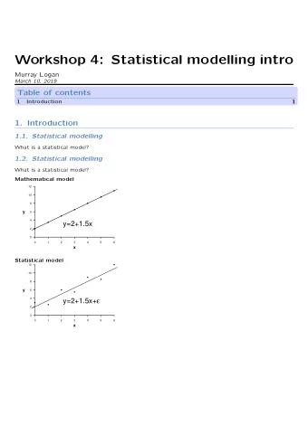
Statistical modelling 12 ● 10 ● ● 8 y 6 ● ● y=2+1.5x+ ε 4 ● ● 2 0 0 1 2 3 4 5 6 x What is a statistical model? • stoichastic mathematical expression • low-dimensional summary • relates one or more dependent random variables to one or more independent variables

Statistical modelling A random variable is one whose values depend on a set of random events and are described by a probability distribution

Statistical modelling 12 ● 10 ● ● 8 y 6 ● ● y=2+1.5x+ ε 4 ● ● 2 0 0 1 2 3 4 5 6 x What is a statistical model? • embodies a data generation process along with the distributional assumptions underlying this generation • incorporates uncertainty • response = model + error • incorporate error (uncertainty)

Statistical modelling 12 ● 10 ● ● 8 y 6 ● ● y=2+1.5x+ ε 4 ● ● 2 0 0 1 2 3 4 5 6 x What is the purpose of statistical modelling? • describe relationships / effects • estimate effects • predict outcomes

Statistical models 12 ● 10 ● ● 8 y 6 ● ● y=2+1.5x+ ε 4 ● ● 2 0 0 1 2 3 4 5 6 x How do we estimate model parameters? - Y ∼ β 0 + β 1 X What criterion do we use to assess best fit? • Depends on how we assume Y is distributed

Statistical models 12 ● 10 ● ● 8 y 6 ● ● y=2+1.5x+ ε 4 ● ● 2 0 0 1 2 3 4 5 6 x If we assume Y is drawn from a normal (gaussian) distribution฀ • Ordinary Least Squares OLS

Estimation • parameters ◦ location (mean) ◦ spread (variance) - uncertainty

Estimation s a r e s q u s t e a L Parameter estimates 6 8 10 12 14 Sum of squares µ =10 ● ● ● ● ● ● ● ● ● ● 6 8 10 12 14 Parameter estimates

Estimation s a t e t i m e s r e s q u a s a s t L e • Minimize sum of the squared residuals • Solve simultaneous equations β 0 × 1 β 1 × 0 ε 1 3 . 0 = + + Y X β 0 × 1 β 1 × 1 ε 1 2 . 5 = + + 3 0 β 0 × 1 β 1 × 2 ε 2 6 . 0 = + + 2.5 1 β 0 × 1 β 1 × 3 ε 3 5 . 5 = + + 6 2 5.5 3 β 0 × 1 β 1 × 4 ε 4 9 . 0 = + + 9 4 8 . 6 = β 0 × 1 + β 1 × 5 + ε 5 8.6 5 β 0 × 1 β 1 × 6 12 . 0 = + + ε 6 12 6

Estimation e s a t t i m e s r e s q u a t s e a s L • Minimize sum of the squared residuals • Solve simultaneous equations Provided data (and residuals) Gaussian 12 ● 10 ● ● 8 y 6 ● ● y=2+1.5x+ ε 4 ● ● 2 0 0 1 2 3 4 5 6 x

Gaussian distribution Probability density function µ = 25, σ 2 = 5 µ = 25, σ 2 = 2 µ = 10, σ 2 = 2 0 5 10 15 20 25 30 35 40 2 σ 2 π e − ( x − µ )2 f ( x | µ , σ 2 ) = 1 2 σ 2 √

Linear model assumptions • Normality • Homogeneity of variance • Linearity • Independence Homogeneity of variance   σ 2 0 0 ··· . .  σ 2  0 . ··· ε i ∼ N ( 0 , σ 2 )   y i = β 0 + β 1 × x i + ε i V = cov =  . .  . . σ 2 � �� � � �� �  . .  ··· Linearity Normality σ 2 0 ··· ··· Zero covariance (=independence)

Linear model assumptions Homogeneity of variance   σ 2 0 0 ··· . .  σ 2  0 . ··· ε i ∼ N ( 0 , σ 2 )   y i = β 0 + β 1 × x i + ε i V = cov =  . .  . . σ 2 � �� � � �� �  . .  ··· Linearity Normality σ 2 0 ··· ··· Zero covariance (=independence) What do we do, if the data do not satisfy the assumptions?

Scale transformations Frequency Frequency 0 10 20 30 40 0.0 0.5 1.0 1.5 2.0 log 10 Leaf length (cm) Leaf length (cm) Logarithmic scale Linear scale 0 10 20 30 40 0.0 0.5 1.0 1.5 2.0 log 10 leaf length (cm) Leaf length (cm)

Linear model y i = β 0 + β 1 x i + ε i • model embodies data generation processes • pertains to: • effects (linear predictor) • distribution

Data types Type Example Distribution Range real, −∞ ≤ x ≥ ∞ Measurements length, weight Gaussian logNormal real, 0 < x ≥ ∞ real, 0 < x ≥ ∞ Gamma Counts Abundance Poisson discrete, 0 ≥ x ≤ ∞ discrete, 0 ≥ x ≤ ∞ Negative Binomial Binary Presence/Absence Binomial discrete, x = 0 , 1 discrete, 0 ≥ x ≤ n Proportions Ratio Binomial Percentages Percent cover Binomial real, 0 ≤ x ≥ 1 real, 0 ≤ x ≥ 1 Beta What about density?

Gamma zero-bound variables with large var. Probability density function µ = 15, σ 2 = 15 (a = 15, s = 1) µ = 15, σ 2 = 30 (a = 7.5, s = 2) µ = 15, σ 2 = 60 (a = 3.75, s = 4) 0 5 10 15 20 25 30 35 40 1 $f(x | s , a ) = ( s a Γ( a )) x ( a − 1) e {− ( x / s ) } $ a shape s scale as as

Poisson distribution Count data Probability density function λ = 25 λ = 15 λ = 3 0 5 10 15 20 25 30 35 40 f ( x | λ ) = e − λ λ x x ! df dispersion

Negative Binomial Count data Probability density function Probability density function µ = 15, ω = 7.5 ( θ = 0.133; σ 2 = 3 µ ) µ = 25, ω = Inf ( θ = 0 ) µ = 15, ω = 3 ( θ = 0.333; σ 2 = 6 µ ) µ = 15, ω = Inf ( θ = 0 ) µ = 15, ω = 1.667 ( θ = 0.6; σ 2 = 10 µ ) µ = 3, ω = Inf ( θ = 0 ) 0 5 10 15 20 25 30 35 40 0 5 10 15 20 25 30 35 40 f ( x | µ , ω ) = Γ( x + ω ) µ x ω ω Γ( ω ) x ! × ( µ + ω ) µ + ω dispersion when

Binomial distribution Proportions or Presence/absence ( n ) p x (1 − p ) n − x f ( x | n , p ) = p µ = np , σ 2 = np (1 − p ) for presence/absence n = 1

Beta Continuous between 0 and 1 Probability density function µ = 0.5, σ 2 = 0.023 (a = 5, b = 5) µ = 0.167, σ 2 = 0.019 (a = 1, b = 5) µ = 0.833, σ 2 = 0.019 (a = 5, b = 1) µ = 0.5, σ 2 = 0.125 (a = 0.5, b = 0.5) 0.00 0.25 0.50 0.75 1.00 Γ( a + b ) Γ( a )Γ( b ) x a − 1 (1 − x ) b − 1 f ( x | a , b ) = a + b , σ 2 = a ab µ = ( a + b ) 2 . ( a + b +1) • must consider zero-one inflated

Generalized linear models Y = β 0 + β 1 x 1 + ... + β p x p + e g ( µ ) = β 0 + β 1 x 1 + ... + β p x p ���� � �� � Link function Systematic • Random component. Y ∼ Dist ( µ , ... ) • Systematic component [ −∞ , ∞ ] • Link function (g () ) g ( µ ) = β 0 + β 1 x 1 + ... + β p x p

Generalized linear models Linear model is just a special case Y = β 0 + β 1 x 1 + ... + β p x p + e g ( µ ) = β 0 + β 1 x 1 + ... + β p x p ���� � �� � Link function Systematic • Random component. Y ∼ N ( µ , σ 2 ) • Systematic component [ −∞ , ∞ ] • Link function (g () ) I ( µ ) = β 0 + β 1 x 1 + ... + β p x p

Generalized linear models Response variable Probability Dis- Canonical Link function Model name tribution Continuous Gaussian identiy: Linear regression measurements µ Gamma verse: Gamma regression 1/ µ Counts Poisson log: Poisson regression / log-linear model log ( µ ) Negative binomial log: Negative binomial regression log ( µ ) Quasi-poisson log: Poisson regression log ( µ ) Binary,proportions Binomial logit: Logistic regression ( ) π log 1 − π probit: Probit regression ∫ α + β . X ( 2 Z 2 ) 1 − 1 exp dZ √ 2 π −∞ complimentary: Logistic regression log ( − log (1 − π )) Quasi-binomial logit: Logistic regression ( ) π log 1 − π Percentages Beta logit: Beta regression ( ) π log 1 − π

OLS Parameter estimates 6 8 10 12 14 Sum of squares µ =10 ● ● ● ● ● ● ● ● ● ● ● ● ● ● ● 6 8 10 12 14 Parameter estimates

Maximum Likelihood 2 σ 2 π e − ( x − µ )2 f ( x | µ , σ 2 ) = 1 2 σ 2 √ 2 ln σ 2 − ∑ 2 ln L ( µ , σ 2 ) = − n 1 i =1 ( x i − µ ) 2 2 ln (2 π ) − n 2 σ 2 Maximum likelihood estimates: ∑ n x = 1 µ = ¯ ˆ i =1 x i n σ 2 = 1 ∑ n x ) 2 ˆ i =1 ( x i − ¯ n

Maximum Likelihood Parameter estimates 6 8 10 12 14 Log−likelihood µ =10 ● ● ● ● ● 6 6 6 8 8 8 10 10 10 12 12 12 14 14 14 Parameter estimates