What we learned last time 1. Intelligence is the computational part - PowerPoint PPT Presentation

What we learned last time 1. Intelligence is the computational part of the ability to achieve goals • looking deeper: 1) its a continuum, 2) its an appearance, 3) it varies with observer and purpose 2. We will (probably) figure out how to make intelligent systems in our lifetimes; it will change everything 3. But prior to that it will probably change our careers • as companies gear up to take advantage of the economic opportunities 4. This course has a demanding workload

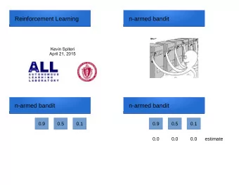
Multi-arm Bandits Sutton and Barto, Chapter 2 The simplest reinforcement learning problem

You are the algorithm! (bandit1) • Action 1 — Reward is always 8 • value of action 1 is q ∗ (1) = 8 • Action 2 — 88% chance of 0, 12% chance of 100! • value of action 2 is q ∗ (2) = . 88 × 0 + . 12 × 100 = 12 • Action 3 — Randomly between -10 and 35, equiprobable q ∗ (3) = 12 . 5 -10 0 35 q ∗ (3) • Action 4 — a third 0, a third 20, and a third from {8,9,…, 18} 0 20 q ∗ (4) q ∗ (4) = 1 3 × 0 + 1 3 × 20 + 1 3 × 13 = 0 + 20 3 + 13 3 = 33 3 = 11

The k -armed Bandit Problem • On each of an infinite sequence of time steps , t =1, 2, 3, …, 
 you choose an action A t from k possibilities, and receive a real- valued reward R t • The reward depends only on the action taken; 
 it is indentically, independently distributed (i.i.d.): q ∗ ( a ) . = E [ R t | A t = a ] , ∀ a ∈ { 1 , . . . , k } true value s • These true values are unknown. The distribution is unknown • Nevertheless, you must maximize your total reward • You must both try actions to learn their values (explore), 
 and prefer those that appear best (exploit)

The Exploration/Exploitation Dilemma • Suppose you form estimates action-value estimates Q t ( a ) ≈ q ∗ ( a ) , ∀ a • Define the greedy action at time t as . A ∗ = arg max Q t ( a ) t a • If then you are exploiting 
 A t = A ∗ t If then you are exploring A t 6 = A ∗ t • You can’t do both, but you need to do both • You can never stop exploring, but maybe you should explore less with time. Or maybe not.

Action-Value Methods • Methods that learn action-value estimates and nothing else • For example, estimate action values as sample averages : P t − 1 i =1 R i · 1 A i = a = sum of rewards when a taken prior to t Q t ( a ) . = P t − 1 number of times a taken prior to t i =1 1 A i = a • The sample-average estimates converge to the true values 
 If the action is taken an infinite number of times N t ( a ) →∞ Q t ( a ) = q ∗ ( a ) lim The number of times action a has been taken by time t

ε -Greedy Action Selection • In greedy action selection, you always exploit • In 𝜁 -greedy, you are usually greedy, but with probability 𝜁 you instead pick an action at random (possibly the greedy action again) • This is perhaps the simplest way to balance exploration and exploitation

A simple bandit algorithm Initialize, for a = 1 to k : Q ( a ) ← 0 N ( a ) ← 0 Repeat forever: ⇢ arg max a Q ( a ) with probability 1 − ε (breaking ties randomly) A ← a random action with probability ε R ← bandit ( A ) N ( A ) ← N ( A ) + 1 1 ⇥ ⇤ Q ( A ) ← Q ( A ) + R − Q ( A ) N ( A )

What we learned last time 1. Multi-armed bandits are a simplification of the real problem 1. they have action and reward (a goal), but no input or sequentiality 2. A fundamental exploitation-exploration tradeoff arises in bandits 1. 𝜁 -greedy action selection is the simplest way of trading off 3. Learning action values is a key part of solution methods 4. The 10-armed testbed illustrates all

One Bandit Task from 
 The 10-armed Testbed q ∗ ( a ) ∼ N (0 , 1) 4 R t ∼ N ( q ∗ ( a ) , 1) 3 q ∗ (3) q ∗ (5) 2 1 q ∗ (9) q ∗ (4) q ∗ (1) Reward 0 q ∗ (7) q ∗ (10) distribution -1 q ∗ (2) q ∗ (8) q ∗ (6) -2 Run for 1000 steps Repeat the whole -3 thing 2000 times with different bandit tasks -4 1 2 3 4 5 6 7 8 9 10 Action

ε -Greedy Methods on the 10-Armed Testbed

What we learned last time 1. Multi-armed bandits are a simplification of the real problem 1. they have action and reward (a goal), but no input or sequentiality 2. The exploitation-exploration tradeoff arises in bandits 1. 𝜁 -greedy action selection is the simplest way of trading off 3. Learning action values is a key part of solution methods 4. The 10-armed testbed illustrates all 5. Learning as averaging – a fundamental learning rule

Averaging ⟶ learning rule • To simplify notation, let us focus on one action • We consider only its rewards, and its estimate after n+ 1 rewards: = R 1 + R 2 + · · · + R n − 1 Q n . . n − 1 • How can we do this incrementally (without storing all the rewards)? • Could store a running sum and count (and divide), or equivalently: Q n +1 = Q n + 1 h i R n − Q n n • This is a standard form for learning/update rules: h i NewEstimate ← OldEstimate + StepSize Target − OldEstimate

Derivation of incremental update = R 1 + R 2 + · · · + R n − 1 Q n . . n − 1 n 1 X = Q n +1 R i n i =1 n − 1 ! 1 X = R n + R i n i =1 n − 1 ! 1 1 X = R n + ( n − 1) R i n − 1 n i =1 1 ⇣ ⌘ = R n + ( n − 1) Q n n 1 ⇣ ⌘ = R n + nQ n − Q n n Q n + 1 h i = R n − Q n , n

Averaging ⟶ learning rule • To simplify notation, let us focus on one action • We consider only its rewards, and its estimate after n+ 1 rewards: = R 1 + R 2 + · · · + R n − 1 Q n . . n − 1 • How can we do this incrementally (without storing all the rewards)? • Could store a running sum and count (and divide), or equivalently: Q n +1 = Q n + 1 h i R n − Q n n • This is a standard form for learning/update rules: h i NewEstimate ← OldEstimate + StepSize Target − OldEstimate

Tracking a Non-stationary Problem • Suppose the true action values change slowly over time • then we say that the problem is nonstationary • In this case, sample averages are not a good idea (Why?) • Better is an “exponential, recency-weighted average”: h i Q n +1 = Q n + α R n − Q n n X = (1 − α ) n Q 1 + α (1 − α ) n − i R i i =1 where α is a constant, step-size parameter , 0 < α ≤ 1 • There is bias due to that becomes smaller over time Q 1

Standard stochastic approximation convergence conditions • To assure convergence with probability 1: ∞ ∞ X X α 2 α n ( a ) = ∞ and n ( a ) < ∞ . n =1 n =1 α n = 1 • e.g., if n α n = n − p , p ∈ (0 , 1) then convergence is 
 α n = 1 • not at the optimal rate: n 2 O (1 / √ n )

Optimistic Initial Values • All methods so far depend on , i.e., they are biased. 
 Q 1 ( a ) So far we have used Q 1 ( a ) = 0 • Suppose we initialize the action values optimistically ( ), 
 Q 1 ( a ) = 5 e.g., on the 10-armed testbed (with ) α = 0 . 1 100% optimistic, greedy Q 0 = 5, = 0 80% 휀 1 realistic, ! -greedy 60% % Q 0 = 0, = 0.1 Optimal 휀 1 action 40% 20% 0% 0 200 400 600 800 1000 Plays Steps

Upper Confidence Bound (UCB) action selection • A clever way of reducing exploration over time • Estimate an upper bound on the true action values • Select the action with the largest (estimated) upper bound s " # log t A t . = argmax Q t ( a ) + c N t ( a ) a UCB c = 2 휀 -greedy 휀 = 0.1 Average reward Steps

Gradient-Bandit Algorithms • Let be a learned preference for taking action a H t ( a ) e H t ( a ) Pr { A t = a } . . = = π t ( a ) , P k b =1 e H t ( b ) H t +1 ( a ) . ⇣ ⌘⇣ ⌘ R t − ¯ = H t ( a ) + α { A t = a } − π t ( a ) R t , ∀ a t 100% = 1 R t . ¯ X R i α = 0.1 t 80% with baseline i =1 α = 0.4 % 60% Optimal α = 0.1 action 40% without baseline α = 0.4 20% 0% 0 250 500 750 1000 Steps

Derivation of gradient-bandit algorithm In exact gradient ascent : = H t ( a ) + α∂ E [ R t ] H t +1 ( a ) . (1) ∂ H t ( a ) , where: X E [ R t ] . = π t ( b ) q ∗ ( b ) , b "X # ∂ E [ R t ] ∂ ∂ H t ( a ) = π t ( b ) q ∗ ( b ) ∂ H t ( a ) b q ∗ ( b ) ∂ π t ( b ) X = ∂ H t ( a ) b � ∂ π t ( b ) X � = q ∗ ( b ) − X t ∂ H t ( a ) , b ∂ π t ( b ) where X t does not depend on b , because P ∂ H t ( a ) = 0. b

∂ E [ R t ] � ∂ π t ( b ) X � ∂ H t ( a ) = q ∗ ( b ) − X t ∂ H t ( a ) b � ∂ π t ( b ) X � = π t ( b ) q ∗ ( b ) − X t ∂ H t ( a ) / π t ( b ) b � � ∂ π t ( A t ) � = E q ∗ ( A t ) − X t ∂ H t ( a ) / π t ( A t ) � � � ∂ π t ( A t ) R t − ¯ = E ∂ H t ( a ) / π t ( A t ) , R t where here we have chosen X t = ¯ R t and substituted R t for q ∗ ( A t ), which is permitted because E [ R t | A t ] = q ∗ ( A t ). For now assume: ∂ π t ( b ) � � ∂ H t ( a ) = π t ( b ) 1 a = b − π t ( a ) . Then: R t − ¯ ⇥� � � � ⇤ = E π t ( A t ) 1 a = A t − π t ( a ) / π t ( A t ) R t R t − ¯ ⇥� �� �⇤ = E 1 a = A t − π t ( a ) . R t R t − ¯ � �� � H t +1 ( a ) = H t ( a ) + α 1 a = A t − π t ( a ) , (from (1), QED) R t

Thus it remains only to show that ∂ π t ( b ) � � ∂ H t ( a ) = π t ( b ) 1 a = b − π t ( a ) . Recall the standard quotient rule for derivatives:  f ( x ) ∂ f ( x ) ∂ x g ( x ) − f ( x ) ∂ g ( x ) � ∂ ∂ x = g ( x ) 2 . ∂ x g ( x ) Using this, we can write...