CS 101.2: Notes for Lecture 2 (Bandit Problems) Andreas Krause - PDF document

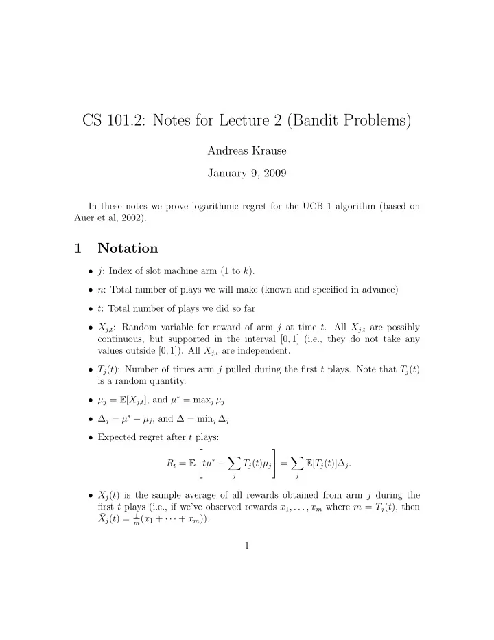
CS 101.2: Notes for Lecture 2 (Bandit Problems) Andreas Krause January 9, 2009 In these notes we prove logarithmic regret for the UCB 1 algorithm (based on Auer et al, 2002). 1 Notation • j : Index of slot machine arm (1 to k ). • n : Total number of plays we will make (known and specified in advance) • t : Total number of plays we did so far • X j,t : Random variable for reward of arm j at time t . All X j,t are possibly continuous, but supported in the interval [0 , 1] (i.e., they do not take any values outside [0 , 1]). All X j,t are independent. • T j ( t ): Number of times arm j pulled during the first t plays. Note that T j ( t ) is a random quantity. • µ j = E [ X j,t ], and µ ∗ = max j µ j • ∆ j = µ ∗ − µ j , and ∆ = min j ∆ j • Expected regret after t plays: � � � � tµ ∗ − R t = E T j ( t ) µ j = E [ T j ( t )]∆ j . j j • ¯ X j ( t ) is the sample average of all rewards obtained from arm j during the first t plays (i.e., if we’ve observed rewards x 1 , . . . , x m where m = T j ( t ), then ¯ X j ( t ) = 1 m ( x 1 + · · · + x m )). 1

2 The Upper Confidence Band algorithm (UCB1) • Initially, play each arm once (hence T j ( t ) ≥ 1 for all t ≥ k ). • Loop (for t = k + 1 to n ) – For each arm j compute “index” v j = ¯ X j ( t ) + c j ( t ) , � log n where c j ( t ) = T j ( t ) . – Play the arm with j ∗ = argmax j v j . 3 Analysis Theorem 1. If UCB 1 is run with input n , then its expected regret R n is O ( K log n ) . ∆ Proof. To prove Theorem 1, we will bound E [ T j ( n )] for all arms j . Suppose, at some time t , UCB 1 pulls a suboptimal arm j . That means, that X j ( t ) + c j ( t ) ≥ ¯ ¯ X ∗ ( t ) + c ∗ ( t ) . Hence, in this case, X ∗ ( t ) + c ∗ ( t ) + ( µ ∗ − µ ∗ ) X j ( t ) + 2 c j ( t ) − c j ( t ) + ( µ j − µ j ) ≥ ¯ ¯ + ( µ j − µ ∗ + 2 c j ( t )) X ∗ ( t ) − ( µ ∗ − c ∗ ( t )) ⇔ ¯ ≥ ¯ X j ( t ) − ( µ j + c j ( t )) � �� � � �� � � �� � − C A B We can see that at least one of A , B or C must be nonnegative, i.e., at least one of the following inequalities must hold: ¯ X j ( t ) ≥ µ j + c j ( t ) (1) X ∗ ( t ) ≤ µ ∗ − c ∗ ( t ) ¯ (2) µ ∗ ≥ µ j + 2 c j ( t ) (3) In order to bound the probability of (1) and (2), we use the Chernoff-Hoeffding inequality: 2

Fact 1 (Chernoff-Hoeffding inequality) . Let X 1 , . . . , X n be independent random vari- ables supported on [0 , 1] , with E [ X i ] = µ . Then, for every a > 0 , n P (1 � X i ≥ µ + a ) ≤ e − 2 a 2 n n i =1 and n P (1 � X i < µ − a ) ≤ e − 2 a 2 n n i =1 Hence, we can bound the probability of (1) as Tj ( t ) T j ( t ) = e − 2 log n = n − 2 . − 2 log n X j ( t ) ≥ µ j + c j ( t )) ≤ e − 2 c j ( t ) 2 T j ( t ) = e P ( ¯ Similarly, X ∗ ( t ) ≤ µ ∗ − c ∗ ( t )) ≤ n − 2 . P ( ¯ Hence, (1) and (2) are very unlikely events. Now, note that whenever T j ( t ) ≥ ℓ = ⌈ (4 log n ) / ∆ 2 j ⌉ , (3) must be false, since � � � log n � log n � ≤ µ j + ∆ j = µ ∗ µ j + 2 c j ( t ) = µ j + 2 T j ( t ) ≤ µ j + 2 4 log n ∆ 2 j Hence, if arm j has been played at least ℓ = O (log n / ∆ 2 j ) times, then inequality (3) must be false, and hence arm j is pulled with probability at most O ( n − 2 ). Now we bound E [ T j ( n )]. By using conditional expectations, we have (writing T j instead of T j ( n ) for short) ≤ ℓ + 2 n − 1 E [ T j ] = P ( T j ≤ ℓ ) E [ T j | T j ≤ ℓ ] + P ( T j ≥ ℓ ) E [ T j | T j ≥ ℓ ] � �� � � �� � � �� � � �� � ≤ 1 ≤ 2 n − 2 ≤ n ≤ ℓ since we have P ( T j ≥ ℓ ) ≤ P (inequality (1) or (2) violated ) ≤ 2 n − 2 . 3

4 Some additional remarks Note that as stated in Section 2, the total number of plays n needs to specified in advance. By setting � 2 log t c t = T j ( t ) , we can avoid this issue. A slightly more complex analysis (of Auer et al ’02) shows that in this case after any number of t plays it holds that R t = O ( k log t ) . ∆ 4