Video Recognition / Optical Flow Various slides from previous - PowerPoint PPT Presentation
CS4501: Introduction to Computer Vision Video Recognition / Optical Flow Various slides from previous courses by: D.A. Forsyth (Berkeley / UIUC), I. Kokkinos (Ecole Centrale / UCL). S. Lazebnik (UNC / UIUC), S. Seitz (MSR / Facebook), J. Hays
CS4501: Introduction to Computer Vision Video Recognition / Optical Flow Various slides from previous courses by: D.A. Forsyth (Berkeley / UIUC), I. Kokkinos (Ecole Centrale / UCL). S. Lazebnik (UNC / UIUC), S. Seitz (MSR / Facebook), J. Hays (Brown / Georgia Tech), A. Berg (Stony Brook / UNC), D. Samaras (Stony Brook) . J. M. Frahm (UNC), V. Ordonez (UVA), Steve Seitz (UW).
Today’s Class • Optical Flow / Video Recognition
Optical Flow Most slides by Juan Carlos Niebles and Ranjay Krishnan Stanford’s Vision Class
Optical Flow Most slides by Juan Carlos Niebles and Ranjay Krishnan Stanford’s Vision Class
From images to videos • A video is a sequence of frames captured over time • Now our image data is a function of space (x, y) and time (t)
Why is motion useful?
Why is motion useful?
Optical flow • Definition: optical flow is the apparent motion of brightness patterns in the image • Note: apparent motion can be caused by lighting changes without any actual motion • Think of a uniform rotating sphere under fixed lighting vs. a stationary sphere under moving illumination Source: Silvio Savarese GOAL: Recover image motion at each pixel from optical flow
Optical flow Vector field function of the spatio-temporal image brightness variations Picture courtesy of Selim Temizer - Learning and Intelligent Systems (LIS) Group, MIT
Estimating optical flow I ( x , y , t –1) I ( x , y , t ) • Given two subsequent frames, estimate the apparent motion field u(x,y), v(x,y) between them • Key assumptions Source: Silvio Savarese • Brightness constancy: projection of the same point looks the same in every frame • Small motion: points do not move very far • Spatial coherence: points move like their neighbors
Key Assumptions: small motions
Key Assumptions: spatial coherence * Slide from Michael Black, CS143 2003
Key Assumptions: brightness Constancy * Slide from Michael Black, CS143 2003
Taylor Series Expansion f ( x ) =
The brightness constancy constraint I ( x , y , t –1) I ( x , y , t ) • Brightness Constancy Equation: I ( x , y , t − 1) = I ( x + u ( x , y ) , y + v ( x , y ), t ) Linearizing the right side using Taylor expansion: Source: Silvio Savarese Image derivative along x I ( x + u , y + v , t ) ≈ I ( x , y , t − 1) + I x ⋅ u ( x , y ) + I y ⋅ v ( x , y ) + I t I ( x + u , y + v , t ) − I ( x , y , t − 1) = I x ⋅ u ( x , y ) + I y ⋅ v ( x , y ) + I t T + I t = 0 × + × + » Hence, I u I v I 0 [ ] → ∇ I ⋅ u v x y t
Filters used to find the derivatives ! " ! $ ! #
The brightness constancy constraint Can we use this equation to recover image motion (u,v) at each pixel? T + I t = 0 [ ] ∇ I ⋅ u v • How many equations and unknowns per pixel? • One equation (this is a scalar equation!), two unknowns (u,v) The component of the flow perpendicular to the gradient (i.e., parallel to the edge) cannot be measured gradient Source: Silvio Savarese ( u , v ) If ( u , v ) satisfies the equation, so does ( u+u’ , v+v’ ) if T = 0 ( u + u ’, v + v ’) [ ] ∇ I ⋅ u ' v ' ( u ’, v ’) edge
The aperture problem Source: Silvio Savarese Actual motion
The aperture problem Source: Silvio Savarese Perceived motion
The barber pole illusion Source: Silvio Savarese http://en.wikipedia.org/wiki/Barberpole_illusion
The barber pole illusion Source: Silvio Savarese http://en.wikipedia.org/wiki/Barberpole_illusion
• Optical flow • Lucas-Kanade method B. Lucas and T. Kanade. An iterative image registration technique with an application to stereo vision. In Proceedings of the International Joint Conference on Artificial Intelligence , pp. 674–679, 1981. Reading: [Szeliski] Chapters: 8.4, 8.5 [Fleet & Weiss, 2005] http://www.cs.toronto.edu/pub/jepson/teaching/vision/2503/opticalFlow.pdf
Solving the ambiguity… B. Lucas and T. Kanade. An iterative image registration technique with an application to stereo vision. In Proceedings of the International Joint Conference on Artificial Intelligence , pp. 674– 679, 1981. • How to get more equations for a pixel? • Spatial coherence constraint: Assume the pixel’s neighbors have the same (u,v) • • If we use a 5x5 window, that gives us 25 equations per pixel Source: Silvio Savarese
Lucas-Kanade flow • Overconstrained linear system: Source: Silvio Savarese
Lucas-Kanade flow • Overconstrained linear system Least squares solution for d given by Source: Silvio Savarese The summations are over all pixels in the K x K window
Conditions for solvability • Optimal (u, v) satisfies Lucas-Kanade equation M = A T A is the second moment matrix ! When is This Solvable? (Harris corner detector…) • A T A should be invertible • A T A should not be too small due to noise Source: Silvio Savarese – eigenvalues l 1 and l 2 of A T A should not be too small • A T A should be well-conditioned – l 1 / l 2 should not be too large ( l 1 = larger eigenvalue) Does this remind anything to you?
Errors in Lukas-Kanade • When our assumptions are violated – Brightness constancy is not satisfied – The motion is not small – A point does not move like its neighbors • window size is too large • what is the ideal window size? * From Khurram Hassan-Shafique CAP5415 Computer Vision 2003
Improving accuracy • Recall our small motion assumption I t-1 (x,y) I t-1 (x,y) • This is not exact – To do better, we need to add higher order terms back in: I t-1 (x,y) • This is a polynomial root finding problem – Can solve using Newton’s method (out of scope for this class) – Lukas-Kanade method does one iteration of Newton’s method • Better results are obtained via more iterations * From Khurram Hassan-Shafique CAP5415 Computer Vision 2003
When do the optical flow assumptions fail? In other words, in what situations does the displacement of pixel patches not represent physical movement of points in space? 1. Well, TV is based on illusory motion – the set is stationary yet things seem to move 2. A uniform rotating sphere – nothing seems to move, yet it is rotating 3. Changing directions or intensities of lighting can make things seem to move – for example, if the specular highlight on a rotating sphere moves. 4. Muscle movement can make some spots on a cheetah move opposite direction of motion. – And infinitely more break downs of optical flow.
Action Classification from Video Recommended Paper to Read:
Action Classification from Video CNN + LSTM over sequence of frames Figure from Carreira & Zisserman, 2018
Recurrent Neural Network Cell ℎ & ℎ " #$$ ! "
Recurrent Neural Network Cell ℎ " = tanh(- .. ℎ & + - .0 ! " ) ℎ & ℎ " #$$ ! "
Recurrent Neural Network Cell 2 " ℎ " ℎ & ℎ " #$$ ℎ " = tanh(- .. ℎ & + - .0 ! " ) ! " 2 " = softmax(- .8 ℎ " )
Recurrent Neural Network Cell ' " ℎ " ℎ & ℎ " #$$ ! "
Recurrent Neural Network Cell e (0.7) , $ = [0.1, 0.05, 0.05, 0.1, 0.7] ℎ $ = [0.1 0.2 0 − 0.3 − 0.1 ] ℎ + = [0 0 0 0 0 0 0 ] !"" ℎ $ = [0.1 0.2 0 − 0.3 − 0.1 ] # $ = [0 0 1 0 0] a b c d e c
Recurrent Neural Network Cell ' " ℎ " ℎ & ℎ " #$$ ! "
Recurrent Neural Network Cell ℎ " ℎ & ℎ " #$$ ! "
(Unrolled) Recurrent Neural Network a t <<space>> ) " ) ' ) ( ℎ " ℎ ' ℎ ( ℎ & ℎ " ℎ ' ℎ ( #$$ #$$ #$$ ! " ! ' ! ( c a t
(Unrolled) Recurrent Neural Network cat likes eating ) " ) ' ) ( ℎ " ℎ ' ℎ ( ℎ & ℎ " ℎ ' ℎ ( #$$ #$$ #$$ ! " ! ' ! ( the cat likes
(Unrolled) Recurrent Neural Network positive / negative sentiment rating ) ℎ ( ℎ & ℎ " ℎ ' ℎ ( #$$ #$$ #$$ ! " ! ' ! ( the cat likes
Action Classification from Video 3D CNN of consecutive frames across time Figure from Carreira & Zisserman, 2018
Action Classification from Video Two Stream CNN: Images + Flow Map Figure from Carreira & Zisserman, 2018
Action Classification from Video Two Stream 3D CNN: Images + Flow Map Figure from Carreira & Zisserman, 2018
Action Classification from Video Results on UCF101 actions Figure from Carreira & Zisserman, 2018
Questions? 46
Recommend
More recommend
Explore More Topics
Stay informed with curated content and fresh updates.
