Minimum-Cost Flow Math 482, Lecture 28 Misha Lavrov April 10, 2020 - PowerPoint PPT Presentation
Introduction Basic solutions Pivoting steps Finding an initial feasible solution Minimum-Cost Flow Math 482, Lecture 28 Misha Lavrov April 10, 2020 Introduction Basic solutions Pivoting steps Finding an initial feasible solution The
Introduction Basic solutions Pivoting steps Finding an initial feasible solution Minimum-Cost Flow Math 482, Lecture 28 Misha Lavrov April 10, 2020
Introduction Basic solutions Pivoting steps Finding an initial feasible solution The min-cost flow problem In this problem, we are given: a network ( N , A ) with no source or sink.
Introduction Basic solutions Pivoting steps Finding an initial feasible solution The min-cost flow problem In this problem, we are given: a network ( N , A ) with no source or sink. A demand d k for every node (as in a supply-demand problem).
Introduction Basic solutions Pivoting steps Finding an initial feasible solution The min-cost flow problem In this problem, we are given: a network ( N , A ) with no source or sink. A demand d k for every node (as in a supply-demand problem). Instead of a capacity c ij for every arc ( i , j ) ∈ A , a cost c ij .
Introduction Basic solutions Pivoting steps Finding an initial feasible solution The min-cost flow problem In this problem, we are given: a network ( N , A ) with no source or sink. A demand d k for every node (as in a supply-demand problem). Instead of a capacity c ij for every arc ( i , j ) ∈ A , a cost c ij . Goal: minimize � ( i , j ) ∈ A c ij x ij while satisfying ∆ k ( x ) = d k for every node k (and x ≥ 0 ).
Introduction Basic solutions Pivoting steps Finding an initial feasible solution The min-cost flow problem In this problem, we are given: a network ( N , A ) with no source or sink. A demand d k for every node (as in a supply-demand problem). Instead of a capacity c ij for every arc ( i , j ) ∈ A , a cost c ij . Goal: minimize � ( i , j ) ∈ A c ij x ij while satisfying ∆ k ( x ) = d k for every node k (and x ≥ 0 ). Example: 2 [ 3 ] 3 [ 5 ] $4 $2 $1 1 [ − 5 ] 4 [ − 1 ] $5 $3 $2 $3 6 [ 1 ] 5 [ − 3 ] $1
Introduction Basic solutions Pivoting steps Finding an initial feasible solution Plan for solving min-cost flow Unlike max-flow problems, min-cost flow problems are commonly solved using the simplex method. (There’s fewer constraints, so the basis is smaller.)
Introduction Basic solutions Pivoting steps Finding an initial feasible solution Plan for solving min-cost flow Unlike max-flow problems, min-cost flow problems are commonly solved using the simplex method. (There’s fewer constraints, so the basis is smaller.) To figure out how to do this, we need to know several things: What a basic solution looks like.
Introduction Basic solutions Pivoting steps Finding an initial feasible solution Plan for solving min-cost flow Unlike max-flow problems, min-cost flow problems are commonly solved using the simplex method. (There’s fewer constraints, so the basis is smaller.) To figure out how to do this, we need to know several things: What a basic solution looks like. How to do a pivoting step.
Introduction Basic solutions Pivoting steps Finding an initial feasible solution Plan for solving min-cost flow Unlike max-flow problems, min-cost flow problems are commonly solved using the simplex method. (There’s fewer constraints, so the basis is smaller.) To figure out how to do this, we need to know several things: What a basic solution looks like. How to do a pivoting step. How to determine the reduced costs of an arc.
Introduction Basic solutions Pivoting steps Finding an initial feasible solution Number of basic variables Our constraints are: F x = d , where F is a | N | × | A | matrix where x ij ’s column has a 1 in row j and a − 1 in row i . d is the vector of demands.
Introduction Basic solutions Pivoting steps Finding an initial feasible solution Number of basic variables Our constraints are: F x = d , where F is a | N | × | A | matrix where x ij ’s column has a 1 in row j and a − 1 in row i . d is the vector of demands. Normally, a basic solution would be given by x = F − 1 B d for some choice of | N | variables B .
Introduction Basic solutions Pivoting steps Finding an initial feasible solution Number of basic variables Our constraints are: F x = d , where F is a | N | × | A | matrix where x ij ’s column has a 1 in row j and a − 1 in row i . d is the vector of demands. Normally, a basic solution would be given by x = F − 1 B d for some choice of | N | variables B . Here, one equation is redundant: assuming � k ∈ N d k = 0, the equations add up to 0 = 0. (If the sum is not 0, there is no solution.)
Introduction Basic solutions Pivoting steps Finding an initial feasible solution Number of basic variables Our constraints are: F x = d , where F is a | N | × | A | matrix where x ij ’s column has a 1 in row j and a − 1 in row i . d is the vector of demands. Normally, a basic solution would be given by x = F − 1 B d for some choice of | N | variables B . Here, one equation is redundant: assuming � k ∈ N d k = 0, the equations add up to 0 = 0. (If the sum is not 0, there is no solution.) So our basis will have | N | − 1 variables, assuming the network is connected. 1 1 If there are two or more subnetworks with no arcs between them, we solve the subproblems separately.
Introduction Basic solutions Pivoting steps Finding an initial feasible solution Spanning trees Definition A spanning tree of ( N , A ) is a choice of | N | − 1 arcs forming a connected subnetwork. (For us, connectivity ignores direction.)
Introduction Basic solutions Pivoting steps Finding an initial feasible solution Spanning trees Definition A spanning tree of ( N , A ) is a choice of | N | − 1 arcs forming a connected subnetwork. (For us, connectivity ignores direction.) 2 3 2 3 1 4 1 4 6 5 6 5 Good Bad!
Introduction Basic solutions Pivoting steps Finding an initial feasible solution Spanning trees Definition A spanning tree of ( N , A ) is a choice of | N | − 1 arcs forming a connected subnetwork. (For us, connectivity ignores direction.) 2 3 2 3 1 4 1 4 6 5 6 5 Good Bad! Claim: | N | − 1 variables form a basis exactly when their arcs make a spanning tree.
Introduction Basic solutions Pivoting steps Finding an initial feasible solution Why spanning trees? Q1. Why is being a spanning tree necessary to be a basis?
Introduction Basic solutions Pivoting steps Finding an initial feasible solution Why spanning trees? Q1. Why is being a spanning tree necessary to be a basis? A1. If there are two pieces, then not all systems F x = d with � k ∈ N d k = 0 have solutions. We must have the d k sum to 0 on each piece!
Introduction Basic solutions Pivoting steps Finding an initial feasible solution Why spanning trees? Q1. Why is being a spanning tree necessary to be a basis? A1. If there are two pieces, then not all systems F x = d with � k ∈ N d k = 0 have solutions. We must have the d k sum to 0 on each piece! Q2. Why is being a spanning tree sufficient to be a basis?
Introduction Basic solutions Pivoting steps Finding an initial feasible solution Why spanning trees? Q1. Why is being a spanning tree necessary to be a basis? A1. If there are two pieces, then not all systems F x = d with � k ∈ N d k = 0 have solutions. We must have the d k sum to 0 on each piece! Q2. Why is being a spanning tree sufficient to be a basis? A2. We have an algorithm (next slide) to find a basic solution using only arcs in a spanning tree.
Introduction Basic solutions Pivoting steps Finding an initial feasible solution Why spanning trees? Q1. Why is being a spanning tree necessary to be a basis? A1. If there are two pieces, then not all systems F x = d with � k ∈ N d k = 0 have solutions. We must have the d k sum to 0 on each piece! Q2. Why is being a spanning tree sufficient to be a basis? A2. We have an algorithm (next slide) to find a basic solution using only arcs in a spanning tree. This will give us an x such that F x = d , but not necessarily x ≥ 0 .
Introduction Basic solutions Pivoting steps Finding an initial feasible solution From a spanning tree to a basic solution To find a basic solution, repeat the following: 1 Pick a node k with only one arc of the spanning tree with unknown flow in/out of k . 2 Solve for that remaining flow to make ∆ k ( x ) = d k .
Introduction Basic solutions Pivoting steps Finding an initial feasible solution From a spanning tree to a basic solution To find a basic solution, repeat the following: 1 Pick a node k with only one arc of the spanning tree with unknown flow in/out of k . 2 Solve for that remaining flow to make ∆ k ( x ) = d k . 2 [ 3 ] 3 [ 5 ] 1 [ − 5 ] 4 [ − 1 ] 6 [ 1 ] 5 [ − 3 ]
Introduction Basic solutions Pivoting steps Finding an initial feasible solution From a spanning tree to a basic solution To find a basic solution, repeat the following: 1 Pick a node k with only one arc of the spanning tree with unknown flow in/out of k . 2 Solve for that remaining flow to make ∆ k ( x ) = d k . 2 [ 3 ] 3 [ 5 ] 5 1 [ − 5 ] 4 [ − 1 ] 6 [ 1 ] 5 [ − 3 ] Solve for x 12 using node 1
Introduction Basic solutions Pivoting steps Finding an initial feasible solution From a spanning tree to a basic solution To find a basic solution, repeat the following: 1 Pick a node k with only one arc of the spanning tree with unknown flow in/out of k . 2 Solve for that remaining flow to make ∆ k ( x ) = d k . 2 [ 3 ] 3 [ 5 ] 2 5 1 [ − 5 ] 4 [ − 1 ] 6 [ 1 ] 5 [ − 3 ] Solve for x 23 using node 2
Recommend
More recommend
Explore More Topics
Stay informed with curated content and fresh updates.

