Variational Methods for Inference based on a paper by Michael Jordan - PowerPoint PPT Presentation

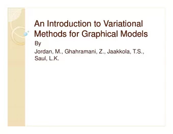
Variational Methods for Inference based on a paper by Michael Jordan et al. Patrick Pletscher ETH Zurich, Switzerland 16th May 2006

The Need for Approximate Methods – FHMM X (1) X (1) X (1) 1 2 3 X (2) X (2) X (2) 1 2 3 X (3) X (3) X (3) 1 2 3 Y 1 Y 2 Y 3 Inference P ( H | E ) = P ( H , E ) complexity O ( N M +1 T ) P ( E ) ,

The Need for Approximate Methods – FHMM X (1) 1 Y 3 Inference P ( H | E ) = P ( H , E ) complexity O ( N M +1 T ) P ( E ) ,

The Need for Approximate Methods – FHMM X (1) 1 Y 3 Inference P ( H | E ) = P ( H , E ) complexity O ( N M +1 T ) P ( E ) ,

Overview 1 Motivation 2 Variational Methods 3 Discussion

Toy Example: ln( x ) Idea of Variational Methods Characterize a probability distribution as the solution of an optimization problem. Intro: ln( x ) variationally Although no probability, still useful. Note ln( x ) is a concave function. ln( x ) = min λ { λ x − ln λ − 1 } ln( x ) now a linear function! Price: minimization has to be carried out for each x . Upper bounds For any given x , we have: ln( x ) ≤ λ x − ln λ − 1 , for all λ .

Toy Example: ln( x ) 5 2.5 ln( x ) ln( x ) 0 − 2.5 − 5 0 0.5 1 1.5 2 2.5 3 x x

Toy Example: ln( x ) 5 2.5 ln( x ) ln( x ) 0 − 2.5 − 5 0 0.5 1 1.5 2 2.5 3 x x

Toy Example: ln( x ) x = 1: d d λ { λ · 1 − ln λ − 1 } ! = 0 it follows: λ = 1

Toy Example: ln( x ) 5 2.5 ln( x ) ln( x ) 0 − 2.5 − 5 0 0.5 1 1.5 2 2.5 3 x x

Toy Example: ln( x ) 5 2.5 ln( x ) ln( x ) 0 − 2.5 − 5 0 0.5 1 1.5 2 2.5 3 x x

Toy Example: ln( x ) 5 2.5 ln( x ) ln( x ) 0 − 2.5 − 5 0 0.5 1 1.5 2 2.5 3 x x

Toy Example: ln( x ) 5 2.5 ln( x ) ln( x ) 0 − 2.5 − 5 0 0.5 1 1.5 2 2.5 3 x x

Toy Example: ln( x ) 5 2.5 ln( x ) ln( x ) 0 − 2.5 − 5 0 0.5 1 1.5 2 2.5 3 x x

Toy Example: ln( x ) 5 2.5 ln( x ) ln( x ) 0 − 2.5 − 5 0 0.5 1 1.5 2 2.5 3 x x

Convex Duality (1/2) 1 Transform function such that it becomes convex or concave . Transformation has to be invertible . 2 Calculate conjugate function (for concave function f ( x )) λ { λ T x − f ∗ ( λ ) } , f ( x ) = min where f ∗ ( λ ) = min x { λ T x − f ( x ) } 3 Transform back.

Convex Duality (2/2) λ x 6 4 2 f ( x ) 0 − 2 1 2 x x

Convex Duality and ln( x ) Example minimize: d dx { λ x − ln( x ) } ! = 0 , we get λ − 1 = 0 → x = 1 ! x λ Finally resubstitute: f ∗ ( λ ) = λ · 1 λ + ln λ = 1 + ln λ Which is the “magical” intercept of the ln example: f ( x ) = min λ { λ x − ln λ − 1 }

Approximations using Convex Duality (1/2) Basic idea Simplify joint probability distribution by transforming the local probability functions. Usually only for “hard” nodes. Afterwards one can use exact methods . This might look like this . . . β γ φ α θ z w θ z N N M M Figure: Replacing a difficult graphical model by a simpler one. Here for Latent Dirichlet Allocation.

Approximations using Convex Duality (2/2) Joint Distribution Product of upper bounds is an upper bound: � P ( S ) = P ( S i | S π ( i ) ) i � P U ( S i | S π ( i ) , λ U ≤ i ) i Marginalization Upper bound for P ( E ), the likelihood: � P ( E ) = P ( H , E ) { H } � � P U ( S i | S π ( i ) , λ U ≤ i ) { H } i

Sequential Approach An unsupervised approach. . . Algorithm transforms nodes, while needed. Backward-“elimination” popular as graph remains tractable. Forward Backward ⇒ ⇒ Discussion • Flexible, out-of-the-box application, • but: no “insider” knowledge is used.

Block Approach A supervised approach. . . Designate in advance which nodes are to be transformed. β γ φ α θ z w θ z N N M M Minimize Kullback-Leibler Divergence λ ∗ = arg min λ D ( Q ( H | E , λ ) � P ( H | E )) , where Q ( S ) ln Q ( S ) � D ( Q � P ) := P ( S ) { S }

FHMM Variationally X (1) X (1) X (1) 1 2 3 X (2) X (2) X (2) 1 2 3 X (3) X (3) X (3) 1 2 3 Y 1 Y 2 Y 3

FHMM Variationally X (1) X (1) X (1) 1 2 3 X (2) X (2) X (2) 1 2 3 X (3) X (3) X (3) 1 2 3 Y 1 Y 2 Y 3

Discussion: some pointers Quite broad questions . . . • Does anybody know more about this new dependence, introduced by the optimization step? • Any theoretical guarantees? • Anybody already used variational methods? If so, for what? Experiences? Junction Tree algorithm . . . • Translation from conditional probabilities to clique potentials? • How do clique potentials change when we introduce the chords?