Variational Inference for GPs: Presenters Group1: Stochastic - - PowerPoint PPT Presentation

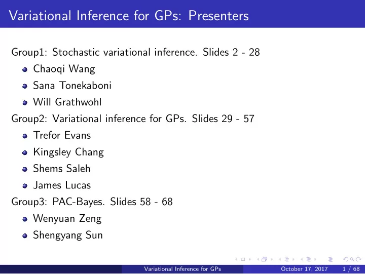
Variational Inference for GPs: Presenters

Group1: Stochastic variational inference. Slides 2 - 28 Chaoqi Wang Sana Tonekaboni Will Grathwohl Group2: Variational inference for GPs. Slides 29 - 57 Trefor Evans Kingsley Chang Shems Saleh James Lucas Group3: PAC-Bayes. Slides 58 - 68 Wenyuan Zeng Shengyang Sun

Variational Inference for GPs October 17, 2017 1 / 68

Variational Inference for GPs

CSC2541 Presentation October 17, 2017

Variational Inference for GPs October 17, 2017 2 / 68

Stochastic Variational Inference, by Matt Hoffman, David M. Blei, Chong Wang, John Paisley

Exponential family and Latent Dirichlet Allocation

Variational Inference for GPs October 17, 2017 3 / 68

Exponential family

Exponential family plays a very important role in statistics and it has many good properties.

1 Most of the commonly used distributions are in the exponential family,

like, Gaussian, multinomial, exponential, Dirichlet, Poisson, Gamma...

2 Also, some are not in the exponential family: Cauchy, uniform... Variational Inference for GPs October 17, 2017 4 / 68

Exponential family: definition

The exponential family is defined as the following form: p(x|η) = exp{ηTT(x) − A(η)}

1 η ∈ Rd, the natural parameters. 2 T : X → Rd, the sufficient statistic. 3 A(η) = ln

• X exp{ηTT(x)}dµ(x), the log normalizer. (µ is the base

measure on a space X) Sometimes, it will be convenient to use a base measure function h(x) : X → R+, and define: p(x|η) = h(x)exp{ηTT(x) − A(η)} , though h can always be included in µ.

Variational Inference for GPs October 17, 2017 5 / 68

Exponential family: examples

Categorical distribution is a discrete probability distribution that describes the possible results of a random event that can be on one of K possible

• utcomes. It is defined as:

1 Parameters: k (#categories); µ1, ..., µk (event probabilities, µi > 0

and µi = 1)

2 Support set: x ∈ {1, ..., k} 3 PMF: p(x) = µx1

1 · · · µxk k , (here, we overload x as

([x = 1], ..., [x = k]))

4 Mode: i when pi = max(µ1, ..., µk) Variational Inference for GPs October 17, 2017 6 / 68

Exponential family: examples

We can write the pmf in the standard representation: p(x|µ) = k

i=1 µxi i = exp{k i=1 xi ln µi}

, where x = (x1, ..., xk)T, and it also can be written as: p(x|µ) = exp{k−1

i=1 xi ln µi + (1 − k−1 i=1 xi) ln(1 − k−1 i=1 µi)}

= exp{k−1

i=1 xi ln( µi 1−k−1

i=1 µi ) + ln(1 − k−1

i=1 µi)}

Now, we can identify that: ηi = ln(

µi 1−

j µj ), T(x) = x, A(η) = ln(1 + k−1

i=1 exp(ηi)), h(x) = 1

Then, p(x|µ) = p(x|η) = 1 · exp{ηTT(x) − A(η)}

Variational Inference for GPs October 17, 2017 7 / 68

Exponential family: property

Exponential family has some properties.

1 DKL(p(x|η1)||p(x|η2)) = (η1 − η2)T∇A(η1) − A(η1) + A(η2) 2 A(η) is convex. 3 ∇A(η) = E[T(x)] ≈ 1

N

• i T(x(i))

4 ∇2A(η) = E[T(x)T(x)T] − E[T(x)]E[T(x)T] = Var[T(x)] Variational Inference for GPs October 17, 2017 8 / 68

Latent Dirichlet Allocation

Latent Dirichlet Allocation (LDA) is a generative probabilistic model for collections of discrete data such as text corpora.

Variational Inference for GPs October 17, 2017 9 / 68

LDA: process

The generative process of LDA model can be summarized as:

1 Draw topics βk from Dirichlet(η, ..., η) for k ∈ {1, ..., K} 2 For each document d ∈ {1, ..., D} : 1

Draw topic proportions θd from Dirichlet(α, ..., α)

2

For each word w ∈ {1, ..., N} :

Draw topic assignment zdn from Multinomial(θd) Draw word wdn from Multinomial(βzdn)

Variational Inference for GPs October 17, 2017 10 / 68

Latent Dirichlet Allocation: notations

There are some notations used in LDA model:

1 wdn is the nth word in dth document. Each word is an element in the

fixed vocabulary of V terms.

2 βk is a V dimensional vector, on a V − 1 simplex. The wth entry in

topic k is βkw

3 θd is the associated topic proportions of dth document. It is a point

• n the K − 1 simplex.

4 zdn indexes the topic from which wdn is drawn. It is assumed that

each word in each document is drawn from a single topic.

Variational Inference for GPs October 17, 2017 11 / 68

LDA: inference

Graphical model representation of LDA. The boxes are plates representing

• replicates. The outer plate represents documents, while the inner plate

represents the repeated choice of topics and words within a document.

1

The joint distribution is: p(θ, z, w|β, α) = p(θ|α) N

n=1 p(zn|θ)p(wn|zn, β)

1Blei, David M.; Ng, Andrew Y.; Jordan, Michael I (January 2003). Lafferty, John,

• ed. ”Latent Dirichlet Allocation”. Journal of Machine Learning Research. 3 (45): pp.
• 9931022. doi:10.1162/jmlr.2003.3.4-5.993

Variational Inference for GPs October 17, 2017 12 / 68

LDA: inference

The key inferential problem that we need to solve in order to use LDA is that of computing the posterior distribution of the hidden variables given a document: p(θ, z|w, α, β) = p(θ,z,w|β,α)

p(w|α,β)

However, the denominator is computationally intractable.

Variational Inference for GPs October 17, 2017 13 / 68

LDA: inference

One way to approximate the posterior is variational inference. In mean-field variational inference, the variational distributions of each variable are in the same family as the complete conditional. We have: p(zdn = k|θd, β1:K,, wdn) ∝ exp{ln θdk + ln βk,wdn}, p(θd|zd) = Dirichlet(α + N

n=1 zdn),

p(βk|z, w) = Dirichlet(η + D

d=1

N

n=1 zk dnwdn)

So, the corresponding variational distributions are: q(zdn) =Multinomial(φdn), for each update: φdn ∝ exp{Ψ(γdk) + Ψ(λk,wdn) − Ψ(

v λkv)} for n ∈ {1, ..., N}

q(θd) = Dirichlet(γd), for each update, γd = α + N

n=1 φdn

q(βk) = Dirichlet(λk), for each update, λk = η + D

d=1

N

n=1 φk dnwdn

Variational Inference for GPs October 17, 2017 14 / 68

LDA: inference

Before updating the topics λ1:K , we need to compute the local variational parameters for every document. This is particularly wasteful in the beginning of the algorithm when, before completing the first iteration, we must analyze every document with randomly initialized topics.

Variational Inference for GPs October 17, 2017 15 / 68

Stochastic Variational Inference, by Matt Hoffman, David M. Blei, Chong Wang, John Paisley

Variational Inference

Variational Inference for GPs October 17, 2017 16 / 68

Variational Inference

Goal: approximate the posterior distribution of a probabilistic model by introducing a distribution over the hidden variables, and optimizing the parameters of that distribution. Our class of models involves: Obsevations x = x1:N Global hidden variables β Local hidden variables z = z1:N Fixed parameters α (For simplicity we assume that they only govern the global hidden variables)

Variational Inference for GPs October 17, 2017 17 / 68

Global vs. Local Hidden Variables

Global hidden variables β : parameters endowed with a prior p(β) Local hidden variables z = z1:N : contains the hidden structure that governs each observation The difference is determined by conditional dependencies: p(xn,zn|x-n, z-n,β,α) = p(xn,zn|β,α) Also, the complete conditional distribution of the hidden variables are in the exponential family q(β|x, z,α) = h(β)exp(ηg(x,z,α)Tt(β)-agηg(x,z,α)) q(znj|xn,znj,β) = h(znj)exp(ηl(xn,znj,β)Tt(znj)-alηl(xn,znj,β))

Variational Inference for GPs October 17, 2017 18 / 68

Mean-field Variational Inference

Mean-field variational inference: a variational inference family where each hidden variable is independent and governed by its own variational parameter λ govern the global variables and φn govern the local variables q(z,β) = q(β|λ)

N

• n=1

J

• j=1

q(znj|φnj) Also, we set q(β|λ) and q(znj|φnj) to be in the same exponential family as the complete conditional distributions p(β|x, z)andp(znj|xn, zn-j,β) q(β|λ) = h(β)expλTt(β)-ag(λ) q(znj|φnj) = h(hnj)expφT

nj t(znj)-al(φnj)

Variational Inference for GPs October 17, 2017 19 / 68

Batch Variational Bayes

L= E[logq(z,β)]-E[logp(x,z,β)] Coordinate update for λ: λ = Eq[ηg(x,z,α)] Coordinate update for φ: φnj = Eq[ηl(xn,zn−j,β)] Therefore, we can optimize our objective function with an easy coordinate ascend and in closed form

Variational Inference for GPs October 17, 2017 20 / 68

Batch Variational Bayes Algorithm

1 Initialize λ(0) randomly 2 Repeat 3 for each local variational parameter φnj do 4 Update φnj,φ(t)

nj = Eq(t−1)[ηl,j(xn,zn−j,β)]

5 End for 6 Update the global variational parameters λ(t) = Eq(t)[ηg(z1:N,x1:N)] Variational Inference for GPs October 17, 2017 21 / 68

Stochastic Variational Inference

Solution: Use a Stcohastic optimization, repeatedly subsample the data to form noisy estimates of the natural gradient of the ELBO ˆ ∇λL= Eφ[ηg(x,z,α)] - λ ˆ ∇φnjL= Eλ,φn−j[ηl(xn,zn−j,β)] - φnj Some benefits of Natural Gradients: The natural gradient points in the direction of steepest ascent in the Riemannian space Converges faster It is cheaper to compute

Variational Inference for GPs October 17, 2017 22 / 68

Stochastic Variational Inference Algorithm

1 Initialize λ(0) randomly 2 Set a step size ρt appropriately 3 Repeat 4 Sample a datapoint xi uniformly from the dataset 5 Update the local variational parameter of the sample as if we were

doing coordinate ascend φ = Eλ(t−1)[ηg(xN

i ,zN i )]

6 Update the current estimate of the global variational parameters

λ(t) = λ(t−1)+ρt ˆ ∇λL = (1-ρt)λ(t−1)+ ρt Eφ[ηg(xN

i ,zN i )]

Variational Inference for GPs October 17, 2017 23 / 68

A Review Of Stochastic Gradient Variational Bayes

Last lecture instroduced Stochastic Gradient Variational Bayes (SGVB). In SGVB, the ELBO: L(φ) = Ex∼D[Eq(z;φ)[log p(x, z) − log q(z|x, φ)]] is

• ptimized via stochastic gradient decent where we estimate ∂L(φ)

∂φ

using monte-carlo samples. In SGVB our estimator is produced via a 2-step hierarchical sampling procedure: We draw a minibatch of data xi (or xi, xj, xk, ...) We draw a minibatch of samples zi ∼ q(zi|xi, φ) We estimate ∂L(φ)

∂φ

≈

∂ ∂φ(log p(xi, zi) − log q(zi|xi, φ))

Where we have reparameterized zi = f (xi, ǫ, φ) with ǫ ∼ p(ǫ). Thus: ∂L(φ)

∂φ

≈

∂ ∂φ(log p(xi, f (xi, ǫ, φ)) − log q(f (xi, ǫ, φ)|xi, φ))

Variational Inference for GPs October 17, 2017 24 / 68

Required Properties

Both SVI and SGVB require certain assumptions to hold before they can be applied SVI: There exists an analytic form of ∂L(φ)

∂φ

for each model paraemter φ. The approximate posterior q(z|φ) must be in the same exponential family as p(z) SGVB: The likelihood p(x, z) must be differentiable wrt z. The approximate posterior q(z|x, φ) must be differentiabe wrt its parameters φ. There exists a differentiable reparameterization f (x, ǫ, φ), ǫ ∼ p(ǫ) such that z = f (x, ǫ, φ) is distributed as q(z|x, φ).

Variational Inference for GPs October 17, 2017 25 / 68

SVI

Benefits: Performs natural gradient decent. Invariant to parameterization. Exponential family provides a rich set of both continuous and discrete data to be modeled. Allows for scalable inference over large datasets. Downsides: Parameters of variational approximation q(z|φ) must be exactly the exponential family parameters limiting complexity of the relationship between q(z|φ) and data x. Analytic Forms of ELBO derivitives are nessesary. q(z|φ) must be in the same exponential family as p(z).

Variational Inference for GPs October 17, 2017 26 / 68

SGVB

Benefits: Weaker Modeling Assumptions can be made. p(x, z) and q(z|φ) need only be differentiable wrt their parameters. Complex, nonlinear relationships between data and latent variables may be learned. Reparameterization allows for low-variance gradient estimates for all model parameters. Allows for scalable inference over large datasets.

Variational Inference for GPs October 17, 2017 27 / 68

SGVB Continued

Downsides: Naive natural gradient decent is intractible in nonlinear probablistic models (although see Dr. Grosse’s recent work for exciting progress towards approximate NGD for neural network models). Not invariant to model parameterization so extra care must be taken to ensure proper results. Reparameterization limits the type of posterior approximations we can use to continuous distributions (like gaussian, laplace). No proof exists showing that reparameterization gradients have lower varaince than score function estimator.

Variational Inference for GPs October 17, 2017 28 / 68

Variational Inference for GPs

Sparse Gaussian Process

Variational Inference for GPs October 17, 2017 29 / 68

Gaussian Processes Review

y = {f (xi) + ǫ}n

i=1,

X = {xi}n

i=1,

xi ∈ Rd A Gaussian process is a collection of random variables, any finite number

• f which have a joint Gaussian distribution. It is completely specified by its

mean and covariance function.

Variational Inference for GPs October 17, 2017 30 / 68

Gaussian Processes Review

y = {f (xi) + ǫ}n

i=1,

X = {xi}n

i=1,

xi ∈ Rd A Gaussian process is a collection of random variables, any finite number

• f which have a joint Gaussian distribution. It is completely specified by its

mean and covariance function. Prior f ∼ N(0, KX,X), [KX,X]i,j = k(xi, xj) Joint Prior y f∗

• ∼ p(y, f∗) = N
• 0,

KX,X + σ2I KX,∗ K∗,X K∗,∗

• Conditional Distribution

f∗|X, y, X∗ ∼ N(E[f∗], cov[f∗]) E[f∗] = (KX,X + σ2I)−1y cov[f∗] = K∗,∗ − K∗,X(KX,X + σ2I)−1KX,∗

Variational Inference for GPs October 17, 2017 30 / 68

Model Selection

Our kernels are typically parameterized by some hyperparameters θ. For example, the squared exponential kernel k(x, z) = exp(−||x−z||2

2/θ2)

Log Marginal likelihood log p(y|θ, σ2, X) = − 1

2 log |KX,X+σ2I|− 1 2yT X (KX,X+σ2I)−1yX− N 2 log(2π)

Requires O(n3) time and O(n2) storage.

Variational Inference for GPs October 17, 2017 31 / 68

Modifying the Joint Prior

p(f, f∗) = N

• 0,

KX,X KX,∗ K∗,X K∗,∗

• We want to modify this joint prior to reduce computational requirements.

Assume f∗, f conditionally independent given set of inducing point locations Z = {zi}m

i=1 and responses u = {ui}m i=1.

p(f, f∗) =

• p(f, f∗, u)du

q(f, f∗) =

• p(f∗|u)q(f|u)p(u)du

we make an approximation to the training conditional p(f|u) ≈ q(f|u)

Variational Inference for GPs October 17, 2017 32 / 68

Fully Independent Training Conditional (FITC)

We approximate the training conditional with an independent distribution (diagonal covariance) p(f|u) = N(KX,ZK−1

X,Zu,

KX,X − QX,X) q(f|u) = N(KX,ZK−1

X,Zu,

diag[KX,X − QX,X]) where QX,X = KX,ZK−1

Z,ZKZ,X. This gives

p(f, f∗) ≈ N

• 0,

QX,X + diag[KX,X − QX,X] QX,∗ Q∗,X Q*,* + diag[K*,* − Q*,*]

• from this, the cost of computing our conditional distribution decreases

from O(n3) → O(m2n) time and from O(n2) → O(mn) storage.

Variational Inference for GPs October 17, 2017 33 / 68

Variational Inference for GPs

Adapted from a presentation by ”Variational Model Selection for Sparse Gaussian Process Regression” Christopher. P. Ley (2016) 2

2http://games.cmm.uchile.cl/media/uploads/posts/SGP_presentation.pdf

Variational learning of inducing variables I

Titsias (2009) proposed a variational lower bound to approximate the true posterior. The ideal inducing variables should serve as sufficient statistics to the

• bservation y.

p(f|fm, y) = p(f|fm) The augmented true posterior p(f, fm|y) factorises as p(f, fm|y) = p(f|fm)p(fm|y)

Variational learning of inducing variables II

The key is that q(f, fm) must satisfy a factorisation that holds for

• ptimal inducing variables:

True : p(f, fm|y) = p(f|fm)p(fm|y) Approximate : q(f, fm) = p(f|fm)φ(fm)

Variational Model Selection for Sparse Gaussian Process Regression

Variational learning of inducing variables III

This gives rise to the variational distribution q(f , f m) = p(f |f m)φ(f m) where φ(f m) is an unconstrained variational distribution over f m We now can use standard variational Bayesian inference where we minimise the Kullback-Leibler divergence KL(q(f , f m)||p(f , f m|y)) Which gives us an equivalent maximum bound on the true log marginal likelihood: FV (Xm, φ(f m)) =

• f ,f m

q(f , f m) log p(y|f )p(f |f m) q(f , f ) df df m

Variational Model Selection for Sparse Gaussian Process Regression

Computation of the variational bound I

FV (Xm, φ(f m)) =

• f ,f m

p(f |f m)φ(f m) log p(y|f )p(f |f m) p(f |f m)φ(f m) df df m =

• f m

φ(f m)

• f

p(f |f m) log p(y|f )df + log p(f m) φ(f m)

• df

=

• f m

φ(f m)

• log G(f m, y) + log p(f m)

φ(f m)

• df m

log G(f m, y) = log[N(y|E[f |f m], σ2

noiseI)] −

1 2σ2

noise

Tr[Cov(f |f m)] E[f |f m] = KnmK −1

mmf m

Cov[f |f m] = Knn − KnmK −1

mmKmn

Bias-Variance Decomposition

• f

p(f|fm)logp(y|f)df =

bias

• log[N(y|E[f|fm], σ2

noiseI)] −

1 2σ2

noise

Tr[Cov(f|fm)]

• variance

Recall that the bias-variance decomposition in L2 loss: Et∼p(t|x)[(y − t)2] = (y − Et∼p(t|x)[t])2

• bias

+ Var[t|x]

variance

Variational Model Selection for Sparse Gaussian Process Regression

Computation of the variational bound II

Merge the logs FV (Xm, φ(f m)) =

• f m

φ(f m)

• log G(f m, y)p(f m)

φ(f m)

• df m

Reverse Jensens’s inequality to maximize wrt φ(f m): FV (Xm) = log

• f m

G(f m, y)p(f m)df m = log

• f m

N(y|αm, σ2

noiseI)p(f m)df m −

1 2σ2

noise

Tr[Cov(f |f m)] = log[N(y|0, σ2

noiseI + KnmK −1 mmKmn)] −

1 2σ2

noise

Tr[Cov(f |f m)] where Cov[f |f m] = Knn − KnmK −1

mmKmn

Variational Model Selection for Sparse Gaussian Process Regression

Variational bound versus PP log likelihood

The traditional projected process (PP or DTC) log likelihood is FP = log

• N(y|0, σ2I + KnmK −1

mmKmn)

• What we obtained is

FV = log

• N(y|0, σ2I + KnmK −1

mmKmn)

• − 1

2σ2 Tr[Knn − KnmK −1

mmKmn]

We got this extra trace term (the total variance of p(f|fm))

Variational Model Selection for Sparse Gaussian Process Regression

Variational bound for model selection

Learning inducing inputs Xm and (σ2, θ) using continuous

• ptimization

Maximize the bound wrt to (Xm, σ2, θ) FV = log

• N(y|0, σ2I + KnmK −1

mmKmn)

• − 1

2σ2 Tr[Knn − KnmK −1

mmKmn]

The first term encourages fitting the data y The second trace term says to minimize the total variance of p(f|fm) The trace Tr[Knn − KnmK −1

mmKmn] can stand on its own as an

• bjective function for sparse GP learning

Variational bound for model selection

When the approximation is the same as the full covariance matrix, i.e. Knn = KnmK −1

mmKmn

Tr[Knn − KnmK −1

mmKmn] = 0

p(f|fm) becomes a delta function We can reproduce the exact GP prediction

Variational Model Selection for Sparse Gaussian Process Regression

Illustrative comparison on Ed Snelson’s toy data

1 2 3 4 5 6 −2 −1.5 −1 −0.5 0.5 1 1.5 2

We compare the traditional PP/DTC log likelihood FP = log

• N(y|0, σ2I + KnmK −1

mmKmn)

• and the bound

FV = log

• N(y|0, σ2I + KnmK −1

mmKmn)

• − 1

2σ2 Tr[Knn − KnmK −1

mmKmn]

We will jointly maximize over (Xm, σ2, θ)

Variational Model Selection for Sparse Gaussian Process Regression

Illustrative comparison

200 training points, red line is the full GP, blue line the sparse GP. We used 8, 10 and 15 inducing points 8 10 15 VAR PP

Variational bound compared to PP likelihood

The variational method (VFE) converges to the full GP model as we increase the number of inducing variables. But PP would not. VFE tends to find smoother distribution than the fill GP when the inducing vairaibles are not enough. PP tends to interpolate the training examples.

Variational Inference for GPs

FITC and VFE Comparison

Variational Inference for GPs October 17, 2017 40 / 68

Overview of the two methods

Negative Log Marginal Likelihood:

Data fit: Penalizes data outside the covariance ellipse Qff + G Complexity penalty: Characterizes the volume of possible datasets compatible with the data fit term. (Occam’s Razor) Trace term: Ensure that objective function is a true lower bound to marginal likelihood of the full GP

Variational Inference for GPs October 17, 2017 41 / 68

Overview

Points of comparison:

1 Noise Variance 2 Number of Inducing Inputs 3 True GP Posterior 4 Optimas Variational Inference for GPs October 17, 2017 42 / 68

Noise Variance

FITC (left) underestimates the noise variance while VFE (right)

• verestimates it

In full GP, we assume homoscedastic (input independent) noise with parameter σ2

n

FITC uses the diagonal term diag(Kff − Qff ) in GFITC as heteroscedastic (input dependent) noise The trace and data fit terms in VFE can be reduced by increasing σ2

n

causing a bias towards overestimation of the noise variance

Variational Inference for GPs October 17, 2017 43 / 68

Number of Inducing Inputs

VFE improves with additional inducing inputs while FITC may ignore them

Variational Inference for GPs October 17, 2017 44 / 68

Number of Inducing Inputs

FITC avoids the penalty of added inducing inputs by clumping them This also means FITC doesn’t recover the full GP even when given enough resources

Variational Inference for GPs October 17, 2017 45 / 68

Local Optima

FITC relies on local optima The minimum found by FITC through clumping still exists in the

• ptimization surface of many inducing points

Optimizing FITC is easier than VFE Optimizing VFE function includes initializing the inducing points with k-means and initially fixing the hyperparameters VFE recognizes a good solution when we initialize it with the FITC solution

Variational Inference for GPs October 17, 2017 46 / 68

Summary

FITC Behaviour

Over-estimation of marginal likelihood Severe under-estimation of noise variance Wasting modelling resources Not recovering true posterior

VFE Behaviour

True bound to the marginal likelihood of full GP Behaves predictably Improves with extra resources Recovers true posterior when possible

FITC remains easier to optimise and gives a good local optima The VFE objective function is recommended since its optimization difficulties can be mitigated by careful initialization, random starts and FITC initialization In practice, it ends up depending on the dataset

Variational Inference for GPs October 17, 2017 47 / 68

Variational Inference for GPs

SVI for GPs

Variational Inference for GPs October 17, 2017 48 / 68

Are sparse GPs enough?

Standard GPs require O(n3) time complexity and O(n2) storage.

Variational Inference for GPs October 17, 2017 49 / 68

Are sparse GPs enough?

Standard GPs require O(n3) time complexity and O(n2) storage. Sparse GPs cut this down to O(nm2) time complexity and O(nm) storage.

Variational Inference for GPs October 17, 2017 49 / 68

Are sparse GPs enough?

Standard GPs require O(n3) time complexity and O(n2) storage. Sparse GPs cut this down to O(nm2) time complexity and O(nm) storage. But we have huge datasets where n is on the order of millions, or billions! How can we hope to fit (even sparse) GPs to datasets of this magnitude?

Variational Inference for GPs October 17, 2017 49 / 68

Stochastic variational inference!

Variational Inference for GPs October 17, 2017 50 / 68

The GP Variational Bound

Titsias, 2009. showed that log p(y|X) = log

• p(y|u)p(u)du

(1) ≥ log

• exp(L1)p(u)du := L2

(2) Where L1 := Ep(f|u)[log p(y|f)]. Remember:

f - Function evaluated at X y - Noisy observation of f u - Value of function evaluated at inducing points (Z)

Variational Inference for GPs October 17, 2017 51 / 68

The GP Variational Bound

Titsias, 2009. showed that log p(y|X) = log

• p(y|u)p(u)du

(1) ≥ log

• exp(L1)p(u)du := L2

(2) Where L1 := Ep(f|u)[log p(y|f)]. Remember:

f - Function evaluated at X y - Noisy observation of f u - Value of function evaluated at inducing points (Z)

We can compute this analytically (as shown before). Posterior can be viewed as ”collapsed” over inducing points

Variational Inference for GPs October 17, 2017 51 / 68

The GP Variational Bound

Titsias, 2009. showed that log p(y|X) = log

• p(y|u)p(u)du

(1) ≥ log

• exp(L1)p(u)du := L2

(2) Where L1 := Ep(f|u)[log p(y|f)]. Remember:

f - Function evaluated at X y - Noisy observation of f u - Value of function evaluated at inducing points (Z)

We can compute this analytically (as shown before). Posterior can be viewed as ”collapsed” over inducing points We need to be explicit about inducing points to do SVI

Variational Inference for GPs October 17, 2017 51 / 68

Requirements for SVI

Marginalisation of u introduces dependencies in the observations. We need to adjust our VIGP regression model to allow us to use SVI...

Variational Inference for GPs October 17, 2017 52 / 68

From a collapsed posterior to global latent variables

We instead treat the inducing points as global latent variables, with variational distribution q(u)

Variational Inference for GPs October 17, 2017 53 / 68

From a collapsed posterior to global latent variables

We instead treat the inducing points as global latent variables, with variational distribution q(u) We then get a new bound which we can use for SVI. log p(y|X) ≥ Eq(u)[L1 + log p(u) − log q(u)] := L3 (3) (Remember, L1 := Ep(f|u)[log p(y|f)])

Variational Inference for GPs October 17, 2017 53 / 68

From a collapsed posterior to global latent variables

We instead treat the inducing points as global latent variables, with variational distribution q(u) We then get a new bound which we can use for SVI. log p(y|X) ≥ Eq(u)[L1 + log p(u) − log q(u)] := L3 (3) (Remember, L1 := Ep(f|u)[log p(y|f)]) The optimal q(u) is Gaussian, which leads to, L3 =

n

• i=1
• log N(yi|ˆ

µ, β−1) + · · ·

• − KL(q(u)||p(u))

(4) Omitting some terms for brevity (see paper).

Variational Inference for GPs October 17, 2017 53 / 68

From a collapsed posterior to global latent variables

We instead treat the inducing points as global latent variables, with variational distribution q(u) We then get a new bound which we can use for SVI. log p(y|X) ≥ Eq(u)[L1 + log p(u) − log q(u)] := L3 (3) (Remember, L1 := Ep(f|u)[log p(y|f)]) The optimal q(u) is Gaussian, which leads to, L3 =

n

• i=1
• log N(yi|ˆ

µ, β−1) + · · ·

• − KL(q(u)||p(u))

(4) Omitting some terms for brevity (see paper). We can write this as a sum over data points allowing SVI!

Variational Inference for GPs October 17, 2017 53 / 68

Inference with this new bound

We perform SVI using natural gradient updates

Variational Inference for GPs October 17, 2017 54 / 68

Inference with this new bound

We perform SVI using natural gradient updates Exponential family leads to a nice form of the updates See the paper for the derived update rules

Variational Inference for GPs October 17, 2017 54 / 68

Inference with this new bound

We perform SVI using natural gradient updates Exponential family leads to a nice form of the updates See the paper for the derived update rules Training updates are now O(m3)!

Variational Inference for GPs October 17, 2017 54 / 68

Inference with this new bound

We perform SVI using natural gradient updates Exponential family leads to a nice form of the updates See the paper for the derived update rules Training updates are now O(m3)! Can also use non-Gaussian likelihoods because of the L3 factorisation. This normally requires approximations.

Variational Inference for GPs October 17, 2017 54 / 68

Experiments I

Each pane shows the posterior of the GP updated per batch. The variational distribution q(u) is shown by the error bars.

Variational Inference for GPs October 17, 2017 55 / 68

Experiments II

Posterior variance of apartment price by postal region.

Variational Inference for GPs October 17, 2017 56 / 68

Summary

We cannot do SVI on the collapsed VI bound.

Variational Inference for GPs October 17, 2017 57 / 68

Summary

We cannot do SVI on the collapsed VI bound. But we can refactorize it.

Variational Inference for GPs October 17, 2017 57 / 68

Summary

We cannot do SVI on the collapsed VI bound. But we can refactorize it. SVI lets us handle big data and can attain the same optimum parameters.

Variational Inference for GPs October 17, 2017 57 / 68

PAC-Bayes

PAC-Bayes

Variational Inference for GPs October 17, 2017 58 / 68

Hoeffding’s Inequality

How can you infer the probability of orange balls?

3Thanks to Hsuan-Tien Lin in National Taiwan University for his example. Variational Inference for GPs October 17, 2017 59 / 68

Hoeffding’s Inequality

How can you infer the probability of orange balls? Sampling!!!

3Thanks to Hsuan-Tien Lin in National Taiwan University for his example. Variational Inference for GPs October 17, 2017 59 / 68

Hoeffding’s Inequality

How can you infer the probability of orange balls? Sampling!!! Assume the real orange probability is µ, the number of balls sampled is N, the sampling orange probability is ν.

3Thanks to Hsuan-Tien Lin in National Taiwan University for his example. Variational Inference for GPs October 17, 2017 59 / 68

Hoeffding’s Inequality

How can you infer the probability of orange balls? Sampling!!! Assume the real orange probability is µ, the number of balls sampled is N, the sampling orange probability is ν. How accurate is your estimation by sampling?

3

3Thanks to Hsuan-Tien Lin in National Taiwan University for his example. Variational Inference for GPs October 17, 2017 59 / 68

Hoeffding’s Inequality

Hoeffding’s Inequality p [|ν − µ| ≥ ǫ] ≤ 2 exp(−2ǫ2N) (5)

Variational Inference for GPs October 17, 2017 60 / 68

Hoeffding’s Inequality

Hoeffding’s Inequality p [|ν − µ| ≥ ǫ] ≤ 2 exp(−2ǫ2N) (5) The statement ν = µ is probably approximately correct (PAC)

Variational Inference for GPs October 17, 2017 60 / 68

Hoeffding’s Inequality

Hoeffding’s Inequality p [|ν − µ| ≥ ǫ] ≤ 2 exp(−2ǫ2N) (5) The statement ν = µ is probably approximately correct (PAC) When the number of samples is big, your estimation can be very

• accurate. Therefore,

you can LEARN from training set! bigger, better!

Variational Inference for GPs October 17, 2017 60 / 68

Hoeffding’s Inequality

Moving on, supposing we have K hypothesis, whose generalization errors are {ei}K

i=1, whose empirical errors are {ˆ

ei}K

i=1, the probability

for discrepency ǫ p(∃i, |ˆ ei − ei| ≥ ǫ) ≤

• i

P(|ˆ ei − ei| ≥ ǫ) ≤ 2K exp(−ǫ2N) (6)

Variational Inference for GPs October 17, 2017 61 / 68

Hoeffding’s Inequality

Moving on, supposing we have K hypothesis, whose generalization errors are {ei}K

i=1, whose empirical errors are {ˆ

ei}K

i=1, the probability

for discrepency ǫ p(∃i, |ˆ ei − ei| ≥ ǫ) ≤

• i

P(|ˆ ei − ei| ≥ ǫ) ≤ 2K exp(−ǫ2N) (6) Equivently, we have log p(∃i, |ˆ ei − ei| ≥

• log(2K) − log(δ)

N ) ≤ δ (7)

Variational Inference for GPs October 17, 2017 61 / 68

Gibbs Classifier Bayes Classifier

Suppose we’re doing a binary classification task. Let x ∈ X and t ∈ {−1, 1}. The model is composed of a latent function x → y(x), and a classification model P(t|y).

Variational Inference for GPs October 17, 2017 62 / 68

Gibbs Classifier Bayes Classifier

Suppose we’re doing a binary classification task. Let x ∈ X and t ∈ {−1, 1}. The model is composed of a latent function x → y(x), and a classification model P(t|y). From the Bayesian viewpoint, the latent function could be parametrized as y(x|w), where w ∼ Q(w)

Variational Inference for GPs October 17, 2017 62 / 68

Gibbs Classifier Bayes Classifier

Gibbs Classifier predicts the output by first sampling w ∼ Q(w), then returning t∗ = sgny(x∗|w) (8)

Variational Inference for GPs October 17, 2017 63 / 68

Gibbs Classifier Bayes Classifier

Gibbs Classifier predicts the output by first sampling w ∼ Q(w), then returning t∗ = sgny(x∗|w) (8) Bayes classifier predicts the output by integrating the distribution of w, namely t∗ = sgnEw∼Q[y(x∗|w)] (9)

Variational Inference for GPs October 17, 2017 63 / 68

Gibbs Classifier Bayes Classifier

Gibbs Classifier predicts the output by first sampling w ∼ Q(w), then returning t∗ = sgny(x∗|w) (8) Bayes classifier predicts the output by integrating the distribution of w, namely t∗ = sgnEw∼Q[y(x∗|w)] (9) Bayes voting classifier predicts the output by integrating the distribution of w and votes, namely t∗ = sgnEw∼Q[sgny(x∗|w)] (10)

Variational Inference for GPs October 17, 2017 63 / 68

PAC-Bayesian theorem (McAllester, 1999)

4 For any data distribution over X × {−1, +1} and an arbitrary posterior

distribution Q(w), we have that the following bound holds, where the probability is over random i.i.d. samples of size n S = {(xS

i , tS i )|i = 1, · · · , n} drawn from the true data distribution:

p [gen(Q) > emp(S, Q) + f (KL[Q||P], n, δ, emp(S, Q)] ≤ δ (11)

4PAC-Bayesian Generalisation Error Bounds for Gaussian Process Classification Variational Inference for GPs October 17, 2017 64 / 68

PAC-Bayesian theorem (McAllester, 1999)

4 For any data distribution over X × {−1, +1} and an arbitrary posterior

distribution Q(w), we have that the following bound holds, where the probability is over random i.i.d. samples of size n S = {(xS

i , tS i )|i = 1, · · · , n} drawn from the true data distribution:

p [gen(Q) > emp(S, Q) + f (KL[Q||P], n, δ, emp(S, Q)] ≤ δ (11)

4PAC-Bayesian Generalisation Error Bounds for Gaussian Process Classification Variational Inference for GPs October 17, 2017 64 / 68

Variational Inference and PAC-Bayesian

Recall variational inference, which training Evidence Lower Bound(ELBO) to optimize the variational posterior. ELBO = EQ(z|x)[logp(x|z)] − KL[Q(z|x)||P(z)] (12) With the reconstruction error, empirical loss tends to be small. With the regularization term, KL divergence cannot be very big. ⇓ VI tends to have good generalization.

Variational Inference for GPs October 17, 2017 65 / 68

Gaussian Process Classification

Given dataset S = {(xi, ti)}N

i=1, a Gaussian Process models the

dependency, p(y) ∼ N(0, K) p(t|y) =

• i

p(ti|yi) (13) According to Bayes formula, the true posterior is as p(y|S) ∝ p(t|y)p(y) (14) Different with GP regression, classification posterior is intractable, which promotes using variational posterior q(y) (Laplace approximation, for example). q(y) = N(K−1α, Σ) (15)

Variational Inference for GPs October 17, 2017 66 / 68

Gaussian Process Classification

Given q (y |S ), predication for testing data x⋆? Assume k = k (x⋆, X), k⋆ = k (x⋆, x⋆). p (y⋆, y |S ) = p (y⋆ |y) q (y|S) p (y⋆ |y) = N

• kTK−1y, k⋆ − kTK−1k
• (16)

Using conditional Gaussian distribution, we have the predicative distribution q (y⋆ |y, S ) = N

• kTα, k⋆ − kT

K−1 − K−1ΣK−1 k

• (17)

KL divergence between q (y) and p(y) gives PAC bound for GP binary classification.

Variational Inference for GPs October 17, 2017 67 / 68

What can PAC do?

Model Selection. (Not accurate, only as a reference)

Variational Inference for GPs October 17, 2017 68 / 68