Data preprocessing Functional Programming and Intelligent Algorithms - PowerPoint PPT Presentation

Data preprocessing Functional Programming and Intelligent Algorithms Que Tran Høgskolen i Ålesund 20th March 2017 1

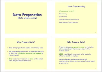
Why data preprocessing? — Real-world data tend to be dirty • incomplete: lacking attribute values, certain attributes of interest, or containing only aggregate data • noisy: containing errors, outlier values • inconsistent: containing discrepancies in codes — "How can the data be preprocessed in order to help improve the quality of the data and, consequently, of the mining results?" 2

Main tasks in Data preprocessing Forms of data preprocessing 3

Data cleaning Data cleaning attempts to: — fill in missing values — smooth noisy data — identify or remove outliers — resolve inconsistencies. 4

Data cleaning Manage missing values: — Ignore the instance — Fill in the missing value manually — Use a global constant to fill in the missing value — Use the attribute mean to fill in the missing value — Use the attribute mean for all instances belonging to the same class as the given instance — Use the most probable value to fill in the missing value 5

Data cleaning Noise data — What is noise ? — Manage noise data: • Binning • Regression • Clustering 6

Data cleaning 7

Data cleaning 8

Data cleaning Manage inconsistent data: — Correct inconsistent data manually using external references — Correct inconsistent data semi-automatically using various tools (Data scrubbing tools, Data auditing tools, Data migration tools...) 9

Data integration — Combines data from multiple sources into a coherent data store — Some important issues: entity identification problem (schema integration, object matching), redundancy, data value conflicts ... 10

Data transformation — The data are transformed into forms appropriate for mining — Data transformation involves: • Generalization • Normalization 11

Data Transformation — Min-max normalization • v ′ = max A − min A ( new _ max A − new _ min A ) + new _ min A v − min A — z-score normalization • v ′ = v − ¯ A σ A 12

Data reduction — Obtain a reduced representation of the data set that is much smaller in volume, yet produce better or (almost) the same analytical results. — Why? • Computational efficiency • Avoid Curse of Dimensionality 13

Curse of Dimensionality High dimension — large volume, sparse data — flexible model — fits training data too well 14

Curse of Dimensionality 15

Data reduction Data reduction involves: — Feature selection — Feature extraction 16

Data reduction Feature selection: — Reduces the data set size by removing irrelevant or redundant features. — Searches for the optimal subset of features — Feature selection methods are typically greedy — Basic heuristic methods include the following techniques: • Stepwise forward selection • Stepwise backward elimination • Combination of forward selection and backward elimination • Decision tree induction 17

Data reduction Feature selection: Greedy (heuristic) methods for attribute subset selection 18

Data reduction Feature extraction: — Reduces the data set size by transforming feature space to lower dimensional space — New features do not tell the same meaning as original features — Data reduction can be lossless or lossy — A popular method: Principle Components Analysis (PCA) 19

Data reduction 20

Data reduction Principal Component Analysis: 1. PCA finds a new basis 2. First axis – the principal component • ... explains most of the variation 3. Next axis chosen perpendicular to previous axes • ... to explain most of the remaining variation 21

Data reduction PCA Algorithm: 1. Write N data points as rows of a matrix X (size N × M ) 2. For each column, subtract its mean to get B 3. Compute covariance C = 1 N B T B 4. Compute eigenvectors and eigenvalues of C • V − 1 CV = D • D : diagonal matrix with eigenvalues • V : matrix of eigenvectors 5. Sort the columns of D in decreasing order of eigenvalues • apply same order to V 6. Discard columns with eigenvalue less than η 7. Transform data by multiplication with V 22