Variance bounds for estimators in autoregressive models with - PowerPoint PPT Presentation

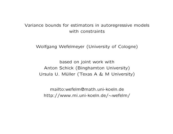
Variance bounds for estimators in autoregressive models with constraints Wolfgang Wefelmeyer (University of Cologne) based on joint work with Anton Schick (Binghamton University) Ursula U. M¨ uller (Texas A & M University) mailto:wefelm@math.uni-koeln.de http://www.mi.uni-koeln.de/ ∼ wefelm/

Let X 1 − p , . . . , X n be observations of a Markov chain of order p , with a parametric model for the conditional mean, E ( X i | X i − 1 ) = r ϑ ( X i − 1 ) , where X i − 1 = ( X i − p , . . . , X i − 1 ) and ϑ is an unknown d -dimensional parameter. An efficient estimator for ϑ in this model is a randomly weighted least squares estimator that solves the estimating equation n � = 0 , σ − 2 ( X i − 1 )˙ � ˜ r ϑ ( X i − 1 ) � X i − r ϑ ( X i − 1 ) i =1 where ˙ r ϑ is the vector of partial derivatives of r ϑ with respect to ϑ , σ 2 ( X i − 1 ) estimates the conditional variance and ˜ σ 2 ( X i − 1 ) = E (( X i − r ϑ ( X i − 1 )) 2 | X i − 1 ) . Aside: The optimal weights are never parametric functions; we al- ways need nonparametric estimators. Wef 1996 AS.

The autoregressive model E ( X i | X i − 1 ) = r ϑ ( X i − 1 ) can be described through its transition distribution A ( x , dy ) = T ( x , dy − r ϑ ( x )) � T ( x , dy ) y = 0 for x = ( x 1 , . . . , x p ). with It can also be written as a nonlinear autoregressive model X i = r ϑ ( X i − 1 ) + ε i with ε i a martingale increment : depends on the past through X i − 1 � T ( x , dy ) y = 0. only and has conditional distribution T ( x , dy ) with We now assume that we know something about the form of T . Then it is useful to describe the model through its transition distribution . Optimal estimators not as weighted least squares but as one-step (Newton–Raphson) estimators. (Possible other approaches: constrained M-estimator, Rao/Wu 2009; empirical likelihood, Owen 2001.)

Our model has transition distribution A ( x , dy ) = T ( x , dy − r ϑ ( x )) with � T ( x , dy ) y = 0 and additional constraint (1) T is partially independent of the past, i.e., T ( x , dy ) = T 0 ( B x , dy ) for a known function B : R p → R q with 0 ≤ q ≤ p . (2) T is invariant under transformation group B j : R p +1 → R p +1 , j = 1 , . . . , m . ( T has density t with t ( z ) = t ( B j z ) for z = ( x , y ).) Optimal estimators for ϑ j (and then jointly) are now constructed differently : First determine Cram´ er–Rao bound and influence func- tion in the least favorable one-dimensional submodel; then construct one-step estimator with this influence function.

Perturb parameter as ϑ nu = ϑ + n − 1 / 2 u , and transition density as t nv ( x , y ) = t ( x , y )(1 + n − 1 / 2 v ( x , y )). The log-likelihood ratio of the observations X d − 1 , . . . , X n is locally asymptotically normal , i.e. ap- proximated by n s uv ( X i − 1 , ε i ) − 1 n − 1 / 2 2 E [ s 2 � uv ( X , ε )] , i =1 where s uv ( x , y ) = u ⊤ ˙ r ( x ) ℓ ( x , y ) + v ( x , y ) with ℓ = − t ′ /t and t ′ ( x , y ) = ∂ y t ( x , y ), and ˙ r = ∂ ϑ r ϑ . The influence function for ϑ j in the least favorable submodel is the gradient of ϑ j , determined as s u ∗ v ∗ such that n 1 / 2 ( ϑ nu,j − ϑ j ) = u = E [ s u ∗ v ∗ ( X , ε ) s uv ( X , ε )] , all u, v. The variance bound is Var s u ∗ v ∗ ( X , ε ). Constraint on t also constrains the possible perturbations v , which leads to different u ∗ and v ∗ .

An efficient estimator ˆ ϑ of ϑ is asymptotically linear with influence function equal to the gradient s u ∗ v ∗ , n ϑ = ϑ + 1 s u ∗ v ∗ ( X i − 1 , ε i ) + o P n ( n − 1 / 2 ) . ˆ � n i =1 A one-step (Newton–Raphson) improvement ˆ ϑ of an initial estimator ˜ ϑ is of the form n ϑ + 1 ε i ) + o P n ( n − 1 / 2 ) ϑ = ˜ ˆ � ˜ s u ∗ v ∗ ( X i − 1 , ˜ n i =1 with ˜ ε i = X i − r ˜ ϑ ( X i − 1 ).

(1) Our model has transition density a ( x , y ) = t ( x , y − r ϑ ( x )) with � yt ( x , dy ) dy = 0 that is partially independent of the past: t ( x , y ) = t 0 ( B x , y ) for a (known) function B : R p → R q with 0 ≤ q ≤ p . The efficient influence function for ϑ is Λ − 1 τ ( x , y ) with score vector r ( X ) − ̺ ( B X )) ℓ 0 ( B X , ε ) + ̺ ( B X ) σ − 2 τ ( X , ε ) = (˙ 0 ( B X ) ε. and information matrix Λ = E [ τ ( X , ε ) τ ⊤ ( X , ε )]. r = ∂ ϑ r ϑ , ℓ 0 = − t ′ 0 /t 0 with t ′ Here ˙ 0 ( x , y ) = ∂ y t 0 ( x , y ), � B x = b ˙ r ϑ ( x ) g ( x ) d x ̺ ( b ) = E (˙ r ( X ) | B X = b ) = , � B x = b g ( x ) d x � y 2 h 0 ( b , y ) dy σ 2 0 ( b ) = E ( ε 2 | B X = b ) = � h 0 ( b , y ) dy , with g and h 0 densities of X and ( B X , ε ). To estimate ϑ efficiently, we therefore need estimators for the efficient score function, i.e. ( p + 1)-dimensional density estimators and (generalized) Nadaraya– Watson estimators. No gain if t 0 ( b , · ) are normal densities.

(2) Our model has transition density a ( x , y ) = t ( x , y − r ϑ ( x )) with � yt ( x , dy ) dy = 0 that is invariant under a group of transformations: t ( z ) = t ( B j z ) for z = ( x , y ) and transformations B j : R p +1 → R p +1 , j = 1 , . . . , m . The efficient influence function for ϑ is Λ − 1 τ ( x , y ) with score vector τ = λ − λ 0 + µ 0 and information matrix Λ = E [ τ ( X , ε ) τ ⊤ ( X , ε )], with symmetrizations m m λ 0 ( z ) = 1 µ 0 ( z ) = 1 � � λ ( B j z ) , µ ( B j z ) m m j =1 j =1 of r ( x ) σ − 2 ( x ) y, λ ( x , y ) = ˙ r ( x ) ℓ ( x , y ) , µ ( x , y ) = ˙ r = ∂ ϑ r ϑ and ℓ = − t ′ /t with t ′ ( x , y ) = ∂ y t ( x , y ), and σ 2 ( x ) = where ˙ E ( ε 2 | X = x ). To estimate ϑ efficiently, we need estimators for these expressions. No gain if t ( b , · ) are normal densities.