Using this on the Z -process we get: 2 ( g ( T i ) g ( T )) 2 T t h - PowerPoint PPT Presentation
European option prices are a good sanity check when analysing bonds with exotic embedded options. Problem: Even with deterministic ZCB-price volatility, B isnt log- normal ( lognormals = lognormal), so it seems we wont
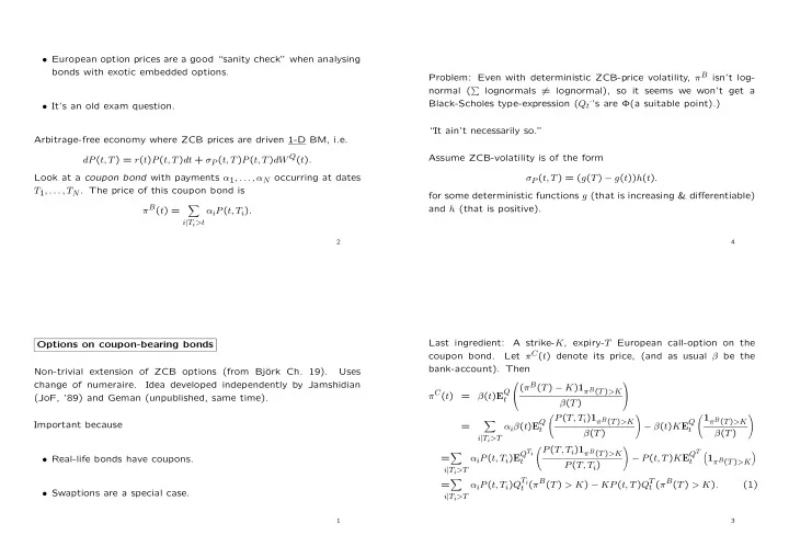
• European option prices are a good “sanity check” when analysing bonds with exotic embedded options. Problem: Even with deterministic ZCB-price volatility, π B isn’t log- normal ( � lognormals � = lognormal), so it seems we won’t get a Black-Scholes type-expression ( Q t · ’s are Φ(a suitable point).) • It’s an old exam question. “It ain’t necessarily so.” Arbitrage-free economy where ZCB prices are driven 1-D BM, i.e. dP ( t, T ) = r ( t ) P ( t, T ) dt + σ P ( t, T ) P ( t, T ) dW Q ( t ) . Assume ZCB-volatility is of the form Look at a coupon bond with payments α 1 , . . . , α N occurring at dates σ P ( t, T ) = ( g ( T ) − g ( t )) h ( t ) . T 1 , . . . , T N . The price of this coupon bond is for some deterministic functions g (that is increasing & differentiable) � π B ( t ) = and h (that is positive). α i P ( t, T i ) . i | T i >t 2 4 Last ingredient: A strike- K , expiry- T European call-option on the Options on coupon-bearing bonds Let π C ( t ) denote its price, (and as usual β be the coupon bond. bank-account). Then Non-trivial extension of ZCB options (from Bj¨ ork Ch. 19). Uses change of numeraire. Idea developed independently by Jamshidian ( π B ( T ) − K ) 1 π B ( T ) >K β ( t ) E Q π C ( t ) = (JoF, ’89) and Geman (unpublished, same time). t β ( T ) � P ( T, T i ) 1 π B ( T ) >K � � 1 π B ( T ) >K � � α i β ( t ) E Q − β ( t ) K E Q Important because = t t β ( T ) β ( T ) i | T i >T � P ( T, T i ) 1 π B ( T ) >K � � � � α i P ( t, T i ) E Q Ti − P ( t, T ) K E Q T = 1 π B ( T ) >K • Real-life bonds have coupons. t t P ( T, T i ) i | T i >T � α i P ( t, T i ) Q T i t ( π B ( T ) > K ) − KP ( t, T ) Q T t ( π B ( T ) > K ) . = (1) • Swaptions are a special case. i | T i >T 1 3
Using this on the Z -process we get: 2 ( g ( T i ) − g ( T )) 2 � T t h 2 ( u ) du + ( g ( T i ) − g ( T )) � T P ( T, T i ) = P ( t, T i ) t h ( u ) dW T ( u ) P ( t, T ) e − 1 Look at the term Q T t ( π B ( T ) > K ) from (1). For each T i define the process Z ( · , T, T i ) Z ( t, T, T i ) = P ( t, T i ) The first term in the “exp” is deterministic. P ( t, T ) By direct application of Theorem 19.8 from Bj¨ ork we have that The stochastic part of the second term, is the same for all T i and � T t h 2 ( u ) du we may write it as putting H ( t, T ) = dZ ( t, T, T i ) = ( g ( T i ) − g ( T )) h ( t ) Z ( t, T, T i ) dW T ( t ) , � where W T is a BM under the T -forward measure. H ( t, T ) X, where X is a N (0 , 1) under Q T and independent of F t . 6 8 Remember that if a process Y solves the stochastic differential equa- tion Note dY ( t ) = µ ( t ; ω ) Y ( t ) dt + σ ( t ; ω ) Y ( t ) dW ( t ) , then for s ≤ t we have • from Proposition 15.5 in Bj¨ ork the forward rate volatility is then �� t � � t s ( µ ( u ; ω ) − 1 σ f ( t, T ) = − ∂ 2 σ 2 ( u ; ω )) du + ∂T σ P ( t, T ) = − g ′ ( T ) h ( t ) , Y ( t ) = Y ( s ) exp s σ ( u ; ω ) dW ( u ) . i.e. it’s deterministic & multiplicatively separable. (Proof: Ito on “what’s inside the exp-function”.) Remember that is σ is deterministic then • this volatility form includes (basically: is ) the Hull/White (ex- � T � T tended Vasicek) model. σ 2 ( u ) du ) , σ ( u ) dW ( u ) ∼ N (0 , t t and independent of F t . 5 7
Remarks All in all we have found that the last term in (1) is The technique will work for other 1-factor models than the Gaussian KP ( t, T )Φ( d ( t, T )) . one (eg. CIR), except you don’t get Φ’s but a more complicated distribution function. How do we find d ( t, T )? We have The technique will not work (without possibly crude approximations) − d ( t, T ) = π − B ( K ) ⇔ π B ( . . . , − d ( t, T )) = π B ( . . . , π − B ( K )) = K, in a multidimensional setting. Why? Well, first so we must find the solution to ax + by = K π B ( . . . , − d ∗ ) = K. defines a line, not a single point. Could try rewriting � a b But π B is a function we know explicitly, that’s easy to do numerically a 2 + b 2 ( a 2 + b 2 x + a 2 + b 2 y ) = K. � � (bisecting or “goal seek”’ing in Excel). � �� � := z 10 12 Repeated use of the relation π B ( T ) π B ( T ; x ) x = X dW τ ( t ) = dW Q ( t ) − σ P ( t, τ ) dt. = � � allows us to perform the same analysis on the Q T i ”a pos. fct”( t, T, T i ) × e ( g ( T i ) − g ( T )) √ t -terms in (1) (this � � � H ( t,T ) × x = . � is DIY) and arrive at: � � x = X i | T i >T Result The time- t price of a call-option on a coupon bearing bond is given by Note that g is increasing and the sum is over i ’s such that T i > T � so g ( T i ) − g ( T ) > 0 and the x �→ π B ( T ; x ) is a monotonely increasing π C ( t ) = α i P ( t, T i )Φ( d ∗ ( t, T i )) − KP ( t, T )Φ( d ∗ ( t, T )) , So it has an inverse function, formally π − B , (with R + as domain). i | T i >T and this function increasing, too. where for any τ ∈ { T, T 1 , . . . , T n } , d ∗ ( t, τ ) is defined implicitly as the solution to the equation We then have H ( t,T )( g ( T i ) − g ( T )) 2 � g ( τ ) − g ( T ) � � g ( Ti ) − g ( T ) − 1 P ( t, T i ) Q T t ( π B ( T ; X ) > K ) = Q T t ( X > π − B ( K )) = Φ( − π − B ( K ) e ( g ( T i ) − g ( T )) H ( t,T ) d ∗ ( t,τ ) = K. ) . 2 α i P ( t, T ) e � �� � := d ( t,T ) i | T i >T 9 11
Simple forward rates; LIBOR A simple forward rate L ( t ; S, T ) specifies the cash-flow for a loan With T = S + δ we may write agreement where L δ ( t ; S ) , L δ ( t ; t ) is called ( δ -) spot LIBOR. • The agreement is made at time t Immediate (Technical) Observation • At time S the borrower receives $1 (or Euro, or DKK, or ...) L δ ( t ; T ) is a Q T + δ martingale. • At time T the borrower pays back 1 + ( T − S ) L ( t ; S, T ) 14 16 But then z would be different for different T i ’s. Then what: You can do various “rank 1”-approximations. Claus Munk has done nice work. Note that this rate is quoted on a discretely compounded basis. If PhD-course participants : How’s that for continuity! L (0; 1 , 1 . 25) = 0 . 04 then you have to pay back 1.01; if the 0.04 were taken as continuously compounded you’d have to pay back exp(0 . 25 ∗ “Topics ...”-course participants : Final project: Implement the for- 0 . 04) = 1 . 010050. mula. Then you could: The usual simple no-arbitrage argument (DIY) shows that • Read the original Jamshidian article. � � 1 + ( T − S ) L ( t ; S, T ) = P ( t, S ) 1 P ( t, S ) P ( t, T ) ⇒ L ( t ; S, T ) = P ( t, T ) − 1 . T − S • Compare theoretical prices of European options to observed Bermu- dan prices (from the embedded options in “realer”). Such simple rates are called LIBOR. • See what Claus does. Replicate his numbers. 13 15
Note that this result is easily extended to any type of floating rate It doesn’t. bond (eg. serial or annuity) with deterministic instalment plan. We have If H ( T i ) denotes remaining principal and A ( T i ) is the principal repaid 1 c i = P ( T i − 1 , T i ) − 1 for i ≤ N − 1 at time T i then N � and the time- t value of the “-1” is of course − P ( t, T i ). Now consider H ( T i − 1 ) = A ( T j ) . the following trading strategy: j = i The T i -cash-flow from the bond is N � • time t : Buy 1 T i − 1 -ZCB (price: P ( t, T i − 1 )) c i = A ( T i )+ δL δ ( T i − 1 ; T i − 1 ) H ( T i − 1 ) = A ( T i )+ δL δ ( T i − 1 ; T i − 1 ) A ( T j ) . j = i A portfolio with A ( T i ) units of the T i -bullet has exactly the same • time T i − 1 : Invest the $1 received in T i -ZCB. You’ll get 1 /P ( T i − 1 , T i ) cash-flows, and its price (assuming t = T 0 ) is � i A ( T i ) = H (0). So units & a net-cash-flow of 0. the new bond has par value too. 18 20 Floating rate bonds & Swaps • time T i : Sit back and receive $ 1 /P ( T i − 1 , T i ) from the T i -ZCB. Look at a tenor-structure; a set of dates where something interesting happens At a cost of P ( t, T i − 1 ), this perfectly replicates the 1 /P ( T i − 1 , T i )-cash- flow from the floating rate bullet. Hence the arbitrage-free price of cash-flow c i is P ( t, T i − 1 ) − P ( t, T i ). The arbitrage-free price of the δ t T 0 floating rate bullet is T 1 = T 0 + δ T i = T i − 1 + δ T N = T 0 + Nδ N − 1 � A floating rate bullet bond has the cash-flows FlBull( t ) = ( P ( t, T i − 1 ) − P ( t, T i )) + P ( T N − 1 ) = P ( t ; T 0 ) , i =1 δL δ ( T i − 1 ; T i − 1 ) at T i for i ≤ N − 1 , and 1+ L δ ( T N − 1 ; T N − 1 ) at date T N . � �� � as the sum telescopes. In particular, if t = T 0 (“vi st˚ ar p˚ a en ter- := c i minsdato”) then the floating rate bullet has value 1. The floating rate The cash-flows are stochastic so finding the arbitrage-free price seems bond has par value. to require a dynamic model. 17 19
Recommend
More recommend
Explore More Topics
Stay informed with curated content and fresh updates.


