Using the Theory of Reals in Analyzing Continuous and Hybrid Systems - PowerPoint PPT Presentation

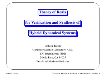
✬ ✩ Using the Theory of Reals in Analyzing Continuous and Hybrid Systems Ashish Tiwari Computer Science Laboratory (CSL) SRI International (SRI) Menlo Park, CA 94025 Email: ashish.tiwari@sri.com ✫ ✪ Ashish Tiwari Reals in Hybrid Systems: 1

✬ ✩ Dynamical Systems A lot of engineering and science concerns dynamical systems • State Space: The set of states, X • Dynamics: The evolutions, T �→ X ◦ Discrete Systems: T is N ◦ Continuous Systems: T is R ◦ Hybrid Systems: T is R × N ✫ ✪ Ashish Tiwari Reals in Hybrid Systems: 2

✬ ✩ Formal Models I Modeling languages: • Continuous systems: Differential equations ◦ The state space formulation x ( t ) ˙ = f ( x ( t ) , u ( t ) , t ) y ( t ) = h ( x ( t ) , t ) x u y • Discrete systems: (Finite) state machines x ′ ) is a formula in some theory ◦ t ( � x, � ✫ ✪ Ashish Tiwari Reals in Hybrid Systems: 3

✬ ✩ Formal Models II Putting the two formal models together, Hybrid Automata: • Embed a continuous dynamical system inside each state • World now evolves in two different ways ◦ Move from one state to another via a discrete transition ◦ Remain in the state and let the continuous world evolve • System has different modes of operation, while some discrete logic performs mode switches X ✫ ✪ Time Ashish Tiwari Reals in Hybrid Systems: 4

✬ ✩ Hybrid Automata A tuple ( Q, X, S 0 , F, Inv , R ) : • Q : finite set of discrete variables • X : finite set of continuous variables • X = ℜ | X | , Q = set of all valuations for Q • S = Q × X • S 0 ⊆ S is the set of initial states • F : Q �→ ( X �→ ℜ | X | ) specifies the rate of flow, ˙ x = F ( q )( x ) • Inv : Q �→ 2 ℜ | X | gives the invariant set • R ⊆ Q × 2 X �→ Q × 2 X captures discontinuous state changes ✫ ✪ Ashish Tiwari Reals in Hybrid Systems: 5

✬ ✩ Hybrid Automata: In picture q = off . x = −kx x < 70 68 < x q = on X . x = M − kx x > 80 x < 82 Time Dense Time: Time does not elapse during discrete transition ✫ ✪ Ashish Tiwari Reals in Hybrid Systems: 6

✬ ✩ Semantics of Hybrid Systems s1 s2 s3 s4 s5 s6 • s 1 ∈ S 0 is an initial state • Discrete Evolution: s i → s i +1 iff R ( s i , s i +1 ) • Continuous Evolution: s i = ( l, x i ) → s i +1 = ( l, x i +1 ) iff there exists a f : ℜ | X | �→ ℜ | X | and δ > 0 such that x i +1 = f ( δ ) x i = f (0) ˙ f = F ( l ) f ( t ) ∈ Inv ( l ) for 0 ≤ t ≤ δ ✫ ✪ Ashish Tiwari Reals in Hybrid Systems: 7

✬ ✩ Questions What can we say (deduce, compute) about the model? x to � x ′ • Reachability. Is there a way to get from state � • Safety. Does the system stay out of a bad region ◦ Can the car ever collide with the car in front? • Liveness. Does something good always happen • Stability. Eventually remain in good region • Timing Properties. Something good happens in 10 seconds Does the model satisfy some property. Property is described in a logic interpreted over the formal models. ✫ ✪ Ashish Tiwari Reals in Hybrid Systems: 8

✬ ✩ Problem • Given a hybrid automata • And a property: safety, reachability, liveness • Show that the property is true of the model • Discrete systems: mc, bmc, abs. inter., inf-bmc, k-induction, deductive rules • Continuous systems: ? • Hybrid systems: ... ✫ ✪ Ashish Tiwari Reals in Hybrid Systems: 9

✬ ✩ Continuous Systems Approach 1: Solve the ODE and eliminate t Eg. If ˙ x = 1 , ˙ y = 1 , then Reach := ∃ t : ( x = x 0 + t ∧ y = y 0 + t ) x = e At � ˙ x = A� � x , then Reach := ∃ t : � x 0 If A is nilpotent: e At x 0 is a polynomial If A has all rational eigenvalues: e At x 0 is a polynomial with e If A has all imaginary rational eigenvalues: e At x 0 is a polynomial with sin , cos In all cases, reduces to ∃ elimination over RCF ✫ ✪ Ashish Tiwari Reals in Hybrid Systems: 10

✬ ✩ Continuous Systems Approach 2: Use inductive invariants cf. Barrier Certificates, Lyapunov Functions Consider the CDS: 0.5 x 1 ˙ = − x 1 − x 2 0 x 2 ˙ = x 1 − x 2 −0.5 x 2 1 + x 2 2 ≤ 0 . 5 is an invariant set. −1 But there are more invariants: −1.5 −2 | x 1 | ≤ 0 . 5 ∧ | x 2 | ≤ 0 . 5 ✫ ✪ −0.5 0 0.5 1 1.5 2 Ashish Tiwari Reals in Hybrid Systems: 11

✬ ✩ Invariants for Dynamical Systems Illustration of invariant sets in 2-D: Invariant Region Box Invariance Box Invariance Arbitrarily shaped Box shaped ✫ ✪ Ashish Tiwari Reals in Hybrid Systems: 12

✬ ✩ Box Invariants A positively invariant rectangular box � l ≤ � x ≤ � u i.e., invariants of the form, l 1 ≤ x 1 ∧ x 1 ≤ u 1 ∧ l 2 ≤ x 2 ∧ x 2 ≤ u 2 ∧ . . . Related Concepts— • Component-wise Asymptotic Stability (CWAS) • Lyapunov stability under the infinity vector norm ✫ ✪ Unstable systems can have useful box invariants Ashish Tiwari Reals in Hybrid Systems: 13

✬ ✩ Why Box Invariants? An Empirical Law for Biological Models: If a model of a biological system is stable, then it also has a rectangular box of attraction—if the system enters this box, then it remains inside it. This “ law” allows verification and parameter estimation for models of biological systems. Natural intuitive meaning ✫ ✪ Ashish Tiwari Reals in Hybrid Systems: 14

✬ ✩ Computing Box Invariants Find Box ( � l, � u ) such that vector field points inwards on the boundary u ) ⇒ dx j ∃ � x ∈ FaceL j ( � � l, � u : ∀ � x : (( � l, � dt ≥ 0) 1 ≤ j ≤ n u ) ⇒ dx j x ∈ FaceU j ( � ∧ ( � l, � dt ≤ 0)) , (1) If dx j dt is a polynomial expression, then existence of box invariants is decidable. ✫ ✪ Ashish Tiwari Reals in Hybrid Systems: 15

✬ ✩ Linear Systems: Deciding Box Invariance A ∈ Q n × n A m = matrix obtained from A s.t. a m ii = a ii , a m ij = | a ij | for i � = j . The following problems are all equivalent and can be solved in O ( n 3 ) time: • Is ˙ � x = A� x strictly box invariant? • Is ˙ x = A m � � x strictly box invariant? z > 0 such that A m � • Is there a � z < 0 ? • Does there exist a positive diagonal matrix D s.t. µ ( D − 1 A m D ) < 0 (in the infinity norm)? • Is − A m a P -matrix? ✫ ✪ Box invariance is stronger than stability for linear systems Ashish Tiwari Reals in Hybrid Systems: 16

✬ ✩ Linear Systems, Box Invariance, Metzler Matrices Matrices with non-negative off-diagonal terms , such as A m , are known as Metzler matrices. A m ∈ R n × n is Metzler and irreducible. Then it has an eigenvalue τ s.t.: 1. τ is real; furthermore, τ > Re ( λ ) , where λ is any other eigenvalue of A m different from τ ; 2. τ is associated with a unique (up to multiplicative constant) positive (right) eigenvector; c > � c ≤ � 0 , such that A m � 3. τ ≤ 0 iff ∃ � 0 ; τ < 0 iff there is at least one strict c ≤ � inequality in A m � 0 ; 4. τ < 0 iff all the principal minors of − A m are positive; 5. τ < 0 iff − ( A m ) − 1 > 0 . ✫ ✪ Ashish Tiwari Reals in Hybrid Systems: 17

✬ ✩ Examples Glucose/Insulin metabolism in Human Body: • Compartmental model of whole body is typically box invariant. • Boxes give bounds on blood sugar concentration in different organs. EGFR / HER2 trafficking model: Proposed affine model is box invariant. Delta-Notch lateral signaling model: The stable modes are box invariants Tetracycline Antibiotics Resistance: ✫ ✪ The resistant mode is box invariant Ashish Tiwari Reals in Hybrid Systems: 18

✬ ✩ Nonlinear Systems d� x = � p ( � x ) dt u ) ⇒ dx j ∃ � x ∈ FaceL j ( � � l, � u : ∀ � x : (( � l, � dt ≥ 0) 1 ≤ j ≤ n u ) ⇒ dx j x ∈ FaceU j ( � ∧ ( � l, � dt ≤ 0)) , (2) If � p are all polynomials, then inductive properties of the form | � x | ≤ c can be computed ✫ ✪ Efficiency is an issue Ashish Tiwari Reals in Hybrid Systems: 19

✬ ✩ Nonlinear Systems: Multiaffine d� x = � p ( � x ) dt Multiaffine: Degree at most one in each variable Example: x 1 x 2 − x 2 x 3 is multiaffine x ∈ Box ( � If p is multiaffine and � l, � u ) , then p ( � x ) is bounded by values of p at vertices of the box Box Invariance Box Invariance ∃∀ (2 n ) to ∃ ( n 2 n ) : ✫ ✪ Generalize: Degree of x j can be arbitrary in p j Ashish Tiwari Reals in Hybrid Systems: 20

✬ ✩ Nonlinear Systems: Monotone Generalize multiaffine systems If f is a monotone function, then f ( � x ) is bounded by values f ( � v ) at the vertices v ˙ � x = � p is monotone if p i is monotone wrt x j for all j � = i . Examples: x = 1 − x 2 is monotone, but not multiaffine ˙ � x = x 3 + x is monotone, but not multiaffine ˙ � ∃∀ (2 n ) to ∃ ( n 2 n ) ✫ ✪ Ashish Tiwari Reals in Hybrid Systems: 21

✬ ✩ Nonlinear Systems: Uniformly Monotone f is uniformly monotone wrt y if it is monotone in the same way for all choices of � x − y Examples: xy − yz is not uniformly monotone wrt y , whereas it is monotonic wrt y xy − yz is uniformly monotone wrt x in domain { y ≥ 0 } ∃∀ (2 n ) to ∃ ( n 2 n ) to ∃ (2 n ) Linear systems are uniformly monotone Linear ⊆ Uniformly monotone ⊆ Monotone ✫ ✪ Ashish Tiwari Reals in Hybrid Systems: 22