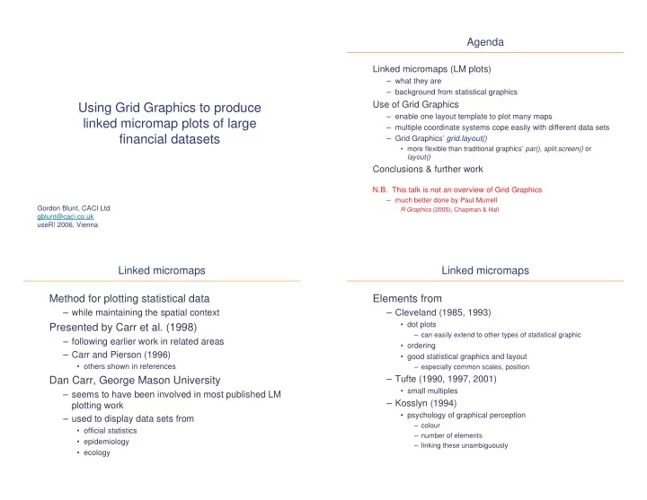
Using Grid Graphics to produce enable one layout template to plot - PowerPoint PPT Presentation

Agenda Linked micromaps (LM plots) – what they are – background from statistical graphics Use of Grid Graphics Using Grid Graphics to produce – enable one layout template to plot many maps linked micromap plots of large – multiple coordinate systems cope easily with different data sets financial datasets – Grid Graphics’ grid.layout() • more flexible than traditional graphics’ par() , split.screen() or layout() Conclusions & further work N.B. This talk is not an overview of Grid Graphics – much better done by Paul Murrell Gordon Blunt, CACI Ltd R Graphics (2005), Chapman & Hall gblunt@caci.co.uk useR! 2006, Vienna Linked micromaps Linked micromaps Method for plotting statistical data Elements from – while maintaining the spatial context – Cleveland (1985, 1993) • dot plots Presented by Carr et al. (1998) – can easily extend to other types of statistical graphic – following earlier work in related areas • ordering – Carr and Pierson (1996) • good statistical graphics and layout • others shown in references – especially common scales, position – Tufte (1990, 1997, 2001) Dan Carr, George Mason University • small multiples – seems to have been involved in most published LM – Kosslyn (1994) plotting work • psychology of graphical perception – used to display data sets from – colour • official statistics – number of elements • epidemiology – linking these unambiguously • ecology

Mean new mortgage value and proportion of mortgages at 95%+ loan-to-value ratio Top right part of plot 2nd Quartile 4th Quartile North Cosby Kilworth Enderby Uppingham Little Mountsorrel Dalby Fleckney Lyndon Leicester Enderby LE 2 2 Coalville Goadby Marwood East East Goscote Goscote Hinckley Barrow Houghton Shepshed on the Hill Stoke Coalville Albany Glenfield Ashby Parva Syston Hinckley Kibworth Birstall Beauchamp Melton Swannington Mowbray Normanton Birstall on Soar Blaby Enderby Leicester Kibworth North LE 3 9 Harcourt Market Ibstock Harborough Kilworth Leicester Ratby LE 1 4 Melton Leicester Mowbray LE 2 3 Stoney Oadby Stanton Loughborough Costock Leicester Uppingham Oadby LE 1 5 Leicester Barrow LE 3 0 upon Soar Leicester Loughborough LE 3 2 Leicester LE 1 3 Thurcaston Leicester Barwell LE 1 7 Little 1st Quartile 3rd Quartile Dalby Leicester Lutterworth LE 2 8 Ashby-de Loughborough la-Zouch Oadby Hinckley Leicester Oakham LE 3 6 Lyndon Ashby-de Blaby la-Zouch Croft Countesthorpe Loughborough Enderby Leicester Cosby LE 4 0 Leicester Humberstone Loughborough Coalville Blaby Birstall Desford Leicester Wigston LE 2 7 Leicester Market LE 2 6 Harborough Leicester 80 100 120 140 160 180 0 10 20 30 Ellistown LE 5 5 Wigston Saxelbye Leicester Leicester LE 1 2 LE 1 1 Mean new mortgage, £000s Prop. 95%+ LTV, % Leicester LE 4 7 Groby Leicester Leicester LE 4 9 Forest East Leicester LE 4 2 Evington Anstey Markfield Leicester Leicester LE 5 0 LE 1 6 Leicester Earl LE 3 1 Shilton Leicester Leicester LE 5 4 LE 2 1 Leicester Hinckley LE 5 3 Leicester Coalville LE 3 5 Leicester Syston LE 4 6 Leicester LE 2 0 Humberstone Leicester Oadby LE 4 5 80 100 120 140 160 180 0 10 20 30 80 100 120 140 160 180 0 10 20 30 Mean new mortgage, £000s Prop. 95%+ LTV, % Mean new mortgage, £000s Prop. 95%+ LTV, % ���������������������������������������������������������������� ��������������������� ������������������������������������� ������������������������������������������������������������������ Key features of linked micromaps grid.layout() , viewports and Grid’s coordinate systems essential 2null Name width 2.5null 2.5null 2mm 2null Name width 2.5null 2.5null Data sorted Chart titles 2.5lines (1, 1) (1, 2) (1, 3) (1, 4) (1, 6) (1, 7) (1, 8) (1, 9) 2.5lines Quartile labels 1lines (2, 1) (2, 2) (2, 3) (2, 4) (2, 6) (2, 7) (2, 8) (2, 9) 1lines – but the map caricatures don’t show data 1null (3, 1) (3, 2) (3, 3) (3, 4) (3, 6) (3, 7) (3, 8) (3, 9) 1null Each column of plots to same scale 1null (4, 1) (4, 2) (4, 3) (4, 4) (4, 6) (4, 7) (4, 8) (4, 9) 1null Simplified boundaries 1null (5, 1) (5, 2) (5, 3) (5, 4) (5, 6) (5, 7) (5, 8) (5, 9) 1null – Dirichlet tesselation for internal boundaries The number of 1null (6, 1) (6, 2) (6, 3) (6, 4) (6, 6) (6, 7) (6, 8) (6, 9) 1null blue rows varies – simplify external boundaries too depending on the 1null (7, 1) (7, 2) (7, 3) (7, 4) (7, 6) (7, 7) (7, 8) (7, 9) 1null number of areas; Legend grid.layout() Quartile labels 1lines (8, 1) (8, 2) (8, 3) (8, 4) (8, 6) (8, 7) (8, 8) (8, 9) 1lines fills the 1null (9, 1) (9, 2) (9, 3) (9, 4) (9, 6) (9, 7) (9, 8) (9, 9) 1null viewport with Small multiples equally sized plotting areas 1null (10, 1) (10, 2) (10, 3) (10, 4) (10, 6) (10, 7) (10, 8) (10, 9) 1null Colour 1null (11, 1) (11, 2) (11, 3) (11, 4) (11, 6) (11, 7) (11, 8) (11, 9) 1null Distort the map if necessary 1null (12, 1) (12, 2) (12, 3) (12, 4) (12, 6) (12, 7) (12, 8) (12, 9) 1null – it spatially indexes the data, it is not accurate geography 1null (13, 1) (13, 2) (13, 3) (13, 4) (13, 6) (13, 7) (13, 8) (13, 9) 1null – e.g. for UK, we typically squash it north – south, move some of Axis text, 2lines (14, 1) (14, 2) (14, 3) (14, 4) (14, 6) (14, 7) (14, 8) (14, 9) 2lines the islands nearer the mainland labels Footnote 1lines (15, 1) (15, 2) (15, 3) (15, 4) (15, 6) (15, 7) (15, 8) (15, 9) 1lines 2null Name width 2.5null 2.5null 2mm 2null Name width 2.5null 2.5null ����������������������������� ���������������!"�����������

Coordinate systems Other Grid features Many coordinate systems are available in Grid Not essential, but useful in our implementation A plot drawn in a Grid viewport fills the viewport We used the following to produce LM plots • the axes are outside the viewport by default native (locations relative to x and y scales of the current viewport) • unless we use plotViewport() npc (normalised parent coordinates) – sets up a central plotting region within a viewport strwidth (string width – for the area names in columns 2 and 7) • LM plots require only one set of axes at the bottom of each column lines (locations specified relative to current font size) of plots mm (millimetres) We’ve found it easier to explain LM plots to clients if each plot is char (locations specified relative to multiples of current font size) separated – slightly – from every other element • have used the width and height arguments to shrink each plot Also, and specific to grid layouts element by a consistent amount null (allows plot elements to be equally sized – by Grid – to fit • in conjunction with npc and native coordinates Grid graphics does this regardless of x and y limits around the areas where the size needs to be fixed) Can place text precisely in viewports There are other coordinate systems too! • or across viewports, if the clip argument is off Conclusions Further work LM plots add insight to our discussions with our clients Different types of statistical graphic have also used (slightly modified) box percentile plots We have adapted Carr et al.’s (1998) methods for see Frank Harrell’s bpplot() , based on Esty and Banfield (2003) displaying financial datasets; the following are crucial used by Dan Carr too … – variables are shown by distance along a linear scale who has also used – they are measured from a common axis time series – the data need to be sorted rates of change – number of points in each plot element needs to be relatively small however, the dot chart seems ideal for LM plots – the plot elements are arranged in small multiples – white gridlines should be used to add guides but not clutter easily understood by my (mostly) non-statistical clients Our functions work for up to 144 areas If the quartile shadings indicate little, or no, spatial pattern: is it possible to plot more? – we might conclude that LM plots are unnecessary I suspect not on A3 paper – so the data could probably be better represented by a simpler this shouldn’t be a limitation method