Using Bayesian Model Probability with ensemble methods to quantify - PowerPoint PPT Presentation
Using Bayesian Model Probability with ensemble methods to quantify uncertainty in reservoir modelling with multiple prior scenarios Sigurd Ivar Aanonsen, NORCE Energy Svenn Tveit, NORCE Energy Mathias Alerini, Equinor ASA EnKF Workshop, Voss,
Using Bayesian Model Probability with ensemble methods to quantify uncertainty in reservoir modelling with multiple prior scenarios Sigurd Ivar Aanonsen, NORCE Energy Svenn Tveit, NORCE Energy Mathias Alerini, Equinor ASA EnKF Workshop, Voss, June 3-5, 2019
Outline ◮ Motivation ◮ Introduction to Bayesian model averaging and selection ◮ Bayesian Model Average (BMA) ◮ Bayesian Model Probability (BMP) ◮ Model Likelihood/Model Evidence (BME) ◮ Bayes Factor (BF) ◮ Calculating BME/BMP ◮ Challenges ◮ Examples ◮ Summary and conclusions
Motivation ◮ Uncertainty quantification in history matching is typically based on a single prior-model scenario. However, often, several alternative models or scenarios are viable a priori. ◮ Geological scenarios, flow scenarios, alternative seismic interpretations, etc.
Motivation ◮ Uncertainty quantification in history matching is typically based on a single prior-model scenario. However, often, several alternative models or scenarios are viable a priori. ◮ Geological scenarios, flow scenarios, alternative seismic interpretations, etc. ◮ Ensemble-based data assimilation methods, like EnKF or ES, does not handle alternative prior models or scenarios. Handling complex model uncertanty is challenging.
Motivation ◮ Uncertainty quantification in history matching is typically based on a single prior-model scenario. However, often, several alternative models or scenarios are viable a priori. ◮ Geological scenarios, flow scenarios, alternative seismic interpretations, etc. ◮ Ensemble-based data assimilation methods, like EnKF or ES, does not handle alternative prior models or scenarios. Handling complex model uncertanty is challenging. ◮ Bayesian theory for models provides a framework for this: ◮ “Total” uncertainty through Bayesian Model Averaging (BMA). ◮ Selecting models or scenarios based on comparing Bayesian Model Probabilities (BMP’s), i.e., probability for a given model or scenario to be correct given the data.
Motivation, cont’d ◮ Bayesian model averaging and model probability rely on the calculation of Bayesian Model Evidence (BME) or Bayes Factors (BF), which have a long history within a number of fields for model comparison and model selection.
Motivation, cont’d ◮ Bayesian model averaging and model probability rely on the calculation of Bayesian Model Evidence (BME) or Bayes Factors (BF), which have a long history within a number of fields for model comparison and model selection. ◮ Few applications to petroleum industry/reservoir modelling (Park et al., 2013, Elsheikh et al., 2014, Hong et al, 2018).
Motivation, cont’d ◮ Bayesian model averaging and model probability rely on the calculation of Bayesian Model Evidence (BME) or Bayes Factors (BF), which have a long history within a number of fields for model comparison and model selection. ◮ Few applications to petroleum industry/reservoir modelling (Park et al., 2013, Elsheikh et al., 2014, Hong et al, 2018). ◮ Recently, it has been shown that, for weakly nonlinear models, Bayesian model selection can be efficiently coupled with ensemble-based data assimilation methods (Carrassi et al., 2017).
Motivation, cont’d ◮ Bayesian model averaging and model probability rely on the calculation of Bayesian Model Evidence (BME) or Bayes Factors (BF), which have a long history within a number of fields for model comparison and model selection. ◮ Few applications to petroleum industry/reservoir modelling (Park et al., 2013, Elsheikh et al., 2014, Hong et al, 2018). ◮ Recently, it has been shown that, for weakly nonlinear models, Bayesian model selection can be efficiently coupled with ensemble-based data assimilation methods (Carrassi et al., 2017). ◮ The methodology can be applied as a “simple” post-processing after having applied standard ensemble-based data assimilation methods to the various scenarios.
Motivation, cont’d ◮ Bayesian model averaging and model probability rely on the calculation of Bayesian Model Evidence (BME) or Bayes Factors (BF), which have a long history within a number of fields for model comparison and model selection. ◮ Few applications to petroleum industry/reservoir modelling (Park et al., 2013, Elsheikh et al., 2014, Hong et al, 2018). ◮ Recently, it has been shown that, for weakly nonlinear models, Bayesian model selection can be efficiently coupled with ensemble-based data assimilation methods (Carrassi et al., 2017). ◮ The methodology can be applied as a “simple” post-processing after having applied standard ensemble-based data assimilation methods to the various scenarios. ◮ However, the use of these methods are disputed. The calculations may be very challenging with respect to e.g. stability, and further investigations of the applicability to reservoir modeling and updating are necessary.
BMA/BMP/BME/BF ◮ Bayesian Model Average (BMA): � P (∆ | D ) = P (∆ | D , M k ) P ( M k | D ) k
BMA/BMP/BME/BF ◮ Bayesian Model Average (BMA): � P (∆ | D ) = P (∆ | D , M k ) P ( M k | D ) k ◮ Bayesian (posterior) Model Probability (BMP): P ( D | M k ) P pri ( M k ) 1 P ( M k | D ) = j P ( D | M j ) P pri ( M j ) = � P ( D | M j ) P pri ( M j ) � j P ( D | M k ) P pri ( M k )
BMA/BMP/BME/BF ◮ Bayesian Model Average (BMA): � P (∆ | D ) = P (∆ | D , M k ) P ( M k | D ) k ◮ Bayesian (posterior) Model Probability (BMP): P ( D | M k ) P pri ( M k ) 1 P ( M k | D ) = j P ( D | M j ) P pri ( M j ) = � P ( D | M j ) P pri ( M j ) � j P ( D | M k ) P pri ( M k ) ◮ Model Likelihood/Model Evidence (BME): � P ( D | M k ) = P ( D | θ, M k ) P ( θ | M k ) d θ Denominator in the “normal” Bayes formula for model k .
BMA/BMP/BME/BF ◮ Bayesian Model Average (BMA): � P (∆ | D ) = P (∆ | D , M k ) P ( M k | D ) k ◮ Bayesian (posterior) Model Probability (BMP): P ( D | M k ) P pri ( M k ) 1 P ( M k | D ) = j P ( D | M j ) P pri ( M j ) = � P ( D | M j ) P pri ( M j ) � j P ( D | M k ) P pri ( M k ) ◮ Model Likelihood/Model Evidence (BME): � P ( D | M k ) = P ( D | θ, M k ) P ( θ | M k ) d θ Denominator in the “normal” Bayes formula for model k . ◮ Bayes factor (BF): BF j - k = P ( D | M j ) P ( D | M k )
Some alternatives for calculating BME 1. Gauss-linear approximation
Some alternatives for calculating BME 1. Gauss-linear approximation P ( D | M k ) = N ( G k θ k , C k ) � − 1 � (( 2 π ) n d det C k ) − 1 / 2 exp 2 ( D − G k θ k ) T C − 1 = ( D − G k θ k ) k C D + G k C θ k G T = C k k � 1 / 2 P ( D | M j ) � det C k � − 1 � ( D − G j θ j ) T C − 1 P ( D | M k ) = exp ( D − G j θ j ) j det C j 2 �� D − G k θ k ) T C − 1 − ( ( D − G k θ k ) k where θ k is prior mean and C k is prior covariance matrix. Utilizing the ensemble representation of the pdf’s, the calculations may be performed in a space of dimension equal to the ensemble size.
Some alternatives for calculating BME 1. Gauss-linear approximation 2. “Inverted Bayes”, i.e., P ( D | M k ) = P ( D | θ, M k ) P ( θ | M k ) P ( θ | D , M k ) using e.g. posterior mean or MAP estimate for θ .
Some alternatives for calculating BME 1. Gauss-linear approximation 2. “Inverted Bayes”, i.e., P ( D | M k ) = P ( D | θ, M k ) P ( θ | M k ) P ( θ | D , M k ) using e.g. posterior mean or MAP estimate for θ .
Alternatives for calculating BME 1. Gauss-linear approximation 2. “Inverted Bayes”, i.e., P ( D | M k ) = P ( D | θ, M k ) P ( θ | M k ) (1) , P ( θ | M k , D ) using e.g. posterior mean or MAP estimate for θ . 3. Importance sampling with posterior ensemble as importance sampler, i.e., averaging Eq. (1) over posterior ensemble.
Alternatives for calculating BME 1. Gauss-linear approximation 2. “Inverted Bayes”, i.e., P ( D | M k ) = P ( D | θ, M k ) P ( θ | M k ) (1) , P ( θ | M k , D ) using e.g. posterior mean or MAP estimate for θ . 3. Importance sampling with posterior ensemble as importance sampler, i.e., averaging Eq. (1) over posterior ensemble. 4. Harmonic average of likelihoods over posterior ensemble (approximation to the importance sampling above): � − 1 � N e 1 1 � P ( D | M k ) ≈ (2) , N e P ( D | θ i , M k ) i = 1
Alternatives for calculating BME 1. Gauss-linear approximation 2. “Inverted Bayes”, i.e., P ( D | M k ) = P ( D | θ, M k ) P ( θ | M k ) (1) , P ( θ | M k , D ) using e.g. posterior mean or MAP estimate for θ . 3. Importance sampling with posterior ensemble as importance sampler, i.e., averaging Eq. (1) over posterior ensemble. 4. Harmonic average of likelihoods over posterior ensemble (approximation to the importance sampling above): � − 1 � N e 1 1 � P ( D | M k ) ≈ (2) , N e P ( D | θ i , M k ) i = 1 5. Eq. 2 with only one realization, i.e., simply the likelihood function (with posterior mean, e.g.).
Challenges ◮ Stability issues: BMP very sensitive to “everything” (amount of data, data mismatch, prior and data covariance matrices, quality of posterior, degree of nonlinearity, ...).
Challenges ◮ Stability issues: BMP very sensitive to “everything” (amount of data, data mismatch, prior and data covariance matrices, quality of posterior, degree of nonlinearity, ...). ◮ Gauss-linear: Nonlinear forward model (BMP mainly depends on prior properties).
Recommend
More recommend
Explore More Topics
Stay informed with curated content and fresh updates.
