Upper confidence bound strategy on stochastical bandits Multiarmed - PDF document

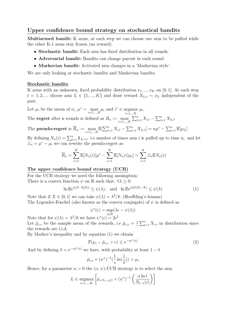
Upper confidence bound strategy on stochastical bandits Multiarmed bandit: K arms, at each step we can choose one arm to be pulled while the other K-1 arms stay frozen (no reward). • Stochastic bandit: Each arm has fixed distribution in all rounds. • Adversarial bandit: Bandits can change payout in each round. • Markovian bandit: Activated arm changes in a ’Markovian style’. We are only looking at stochastic bandits and Markovian bandits. Stochastic bandits K arms with an unknown, fixed probability distribution ν 1 , ..., ν K on [0 , 1]. At each step t = 1 , 2 , ... choose arm I t ∈ { 1 , ..., K } and draw reward X I t ,t ∼ ν I t independent of the past. Let µ i be the mean of ν i , µ ∗ = max i =1 ,...,K µ i and i ∗ ∈ argmax µ i . i =1 ,..,K � n t =1 X i,t − � n The regret after n rounds is defined as R n := max t =1 X I t ,t i =1 ,...,K t =1 X I t ,t ] = nµ ∗ − � n i =1 ,...,K E [ � n t =1 X i,t − � n The pseudo-regret is R n := max t =1 E [ µ I t ] By defining N n ( i ) = � s t =1 ✶ I t = i , i.e number of times arm i is pulled up to time n , and let △ i = µ ∗ − µ i we can rewrite the pseudo-regret as K K K E [ N n ( i )] µ ∗ − � � � R n = E [ N n ( i ) µ i ] = △ i E N n ( i ) i =1 i =1 i =1 The upper confidence bound strategy (UCB) For the UCB strategy we need the following assumption: There is a convex function ψ on R such that, ∀ λ ≥ 0: ln E e λ ( X − E [ X ]) ≤ ψ ( λ ) , ln E e λ ( E [ X ] − X ) ≤ ψ ( λ ) and (1) Note that if X ∈ [0 , 1] we can take ψ ( λ ) = λ 2 / 8. (Hoeffding’s lemma) The Legendre-Fenchel (also known as the convex conjugate) of ψ is defined as ψ ∗ ( ǫ ) = sup ( λǫ − ψ ( λ )) λ ∈ R Note that for ψ ( λ ) = λ 2 / 8 we have ψ ∗ ( ǫ ) = 2 ǫ 2 µ i,s = 1 � s Let ˆ µ i,s be the sample mean of the rewards, i.e ˆ t =1 X i,s in distribution since s the rewards are i.i.d. By Markov’s inequality and by equation (1) we obtain µ i,s > ǫ ) ≤ e − sψ ∗ ( ǫ ) P ( µ i − ˆ (2) And by defining δ = e − sψ ∗ ( ǫ ) we have, with probability at least 1 − δ µ i,s + ( ψ ∗ ) − 1 (1 s ln(1 ˆ δ )) > µ i Hence, for a parameter α > 0 the ( α, ψ )-UCB strategy is to select the arm � α ln t � �� µ i,N t − 1 ( i ) + ( ψ ∗ ) − 1 I t ∈ argmax ˆ N t − 1 ( i ) i =1 ,...,K

Theorem (Pseudo-regret for UCB strategy): Assume that the ν i satisfy the convex assumption (1). Then the pseudo-regret for a ( α, ψ )-UCB stategy with α > 2 satisfies � � α △ i α � R n ≤ ψ ∗ ( △ i / 2) ln n + α − 2 i : △ i > 0 If we have X ∈ [0 , 1], using ψ ∗ ( ǫ ) = 2 ǫ 2 , then � 2 α α � � R n ≤ ln n + △ i α − 2 i : △ i > 0 Lower bound for Bernoulli-distributed rewards For the following result, we are assuming that X i,t ∼ Bernoulli ( p, q ) with p, q ∈ [0 , 1] Theorem (Lower bound): Assume E N n ( i ) = o ( n a ) for a > 0 and that △ i > 0 ∀ i . Then we have R n △ i � lim inf ln n ≥ kl ( µ i , µ ∗ ) n →∞ i : △ i > 0 � � � � µ i 1 − µ i where kl ( µ i , µ ∗ ) = µ i ln + (1 − µ i ) ln is the Kullback-Leibler divergence. 1 − µ ∗ µ ∗ Comparision of lower & upper bound We have that kl ( µ i , µ ∗ ) ≤ ( µ ∗ − µ i ) 2 µ ∗ (1 − µ ∗ ) which follows from ln x ≤ x − 1 . Hence, the lower bound satisfies µ ∗ (1 − µ ∗ ) R n � lim inf ln n ≥ ( µ ∗ − µ i ) n →∞ i : µ ∗ − µ i > 0 Comparing this with the upper bound � 2 α α � � R n ≤ ln n + µ ∗ − µ i α − 2 i : µ ∗ − µ i > 0 we see that the difference between upper and lower bound for a Bernoulli-distributed reward is given by some constants. Page 2

Markovian bandits Again we consider K arms, at each step we can choose one arm to be pulled while the remaining K-1 arms stay frozen. But now the rewards of the pulled arm can change its state in a ’Markovian style’, i.e the arm produces reward r ( x t ) and changes start to x t +1 according to a Markov dynamic x → y with P ( x, y ) The goal now it to maximize a β -discounted reward � ∞ � � r i t ( x i t ( t )) β t E t =0 where i t is the arm pulled at time t and 0 < β < 1 is the discounting factor. This discounted reward is maximized by forward induction. It can be shown (not part of the talk) that the biggest Gittins index �� τ − 1 � t =0 r i ( x i ( t )) β t | x i (0) = x i E G i ( x i ) = sup , where τ is a stopping time, �� τ − 1 � t =0 β t | x i (0) = x i E τ ≥ 1 is enough to determine which arm is to be pulled. Note that the numerator denotes the discounted rewards up to τ and the denumerator represents the discounted time up to τ . Hence, we can find the best strategy by computing the Gittins Index for all arms, where each index is independent of all other arms. Thus, we only need to solve a K-dimensional problem in each step, which greatly reduces the computational work. Page 3