Introduction to Bandits R emi Munos SequeL project: Sequential - PowerPoint PPT Presentation
Introduction to bandits Games Hierarchical bandits Lipschitz optimization X -armed bandits Planning Conclusion Introduction to Bandits R emi Munos SequeL project: Sequential Learning http://researchers.lille.inria.fr/ munos/ INRIA
Introduction to bandits Games Hierarchical bandits Lipschitz optimization X -armed bandits Planning Conclusion Introduction to Bandits R´ emi Munos SequeL project: Sequential Learning http://researchers.lille.inria.fr/ ∼ munos/ INRIA Lille - Nord Europe ThRaSH’2012, Lille, May 2nd, 2012 . . . . . .
Introduction to bandits Games Hierarchical bandits Lipschitz optimization X -armed bandits Planning Conclusion Introduction Multi-armed bandit: simple mathematical model for decision-making under uncertainty. Illustrates the exploration-exploitation tradeoff that appears in any optimization problem where information is missing. Applications: • Clinical trials (Thompson, 1933) • Ads placement on webpages • Computation of Nash equilibria (trafic or communication networks, agent simulation, poker, ...) • Game-playing computers (Go, urban rivals, ...) • Packet routing, itinerary selection, ... • Stochastic optimization under finite numerical budget, ... . . . . . .
Introduction to bandits Games Hierarchical bandits Lipschitz optimization X -armed bandits Planning Conclusion A few references on bandits (2005-2011) [Abbasi-Yadkori, 2009] [Abernethy, Hazan, Rakhlin, 2008] [Abernethy, Bartlett, Rakhlin, Tewari, 2008] [Abernethy, Agarwal, Bartlett, Rakhlin, 2009] [Audibert, Bubeck, 2010] [Audibert, Munos, Szepesv´ ari, 2009] [Audibert, Bubeck, Lugosi, 2011] [Auer, Ortner, Szepesv´ ari, 2007] [Auer, Ortner, 2010] [Awerbuch, Kleinberg, 2008] [Bartlett, Hazan, Rakhlin, 2007] [Bartlett, Dani, Hayes, Kakade, Rakhlin, Tewari, 2008] [Bartlett, Tewari, 2009] [Ben-David, Pal, Shalev-Shwartz, 2009] [Blum, Mansour, 2007] [Bubeck, 2010] [Bubeck, Munos, 2010] [Bubeck, Munos, Stoltz, 2009] [Bubeck, Munos, Stoltz, Szepesv´ ari, 2008] [Cesa-Bianchi, Lugosi, 2006] [Cesa-Bianchi, Lugosi, 2009] [Chakrabarti, Kumar, Radlinski, Upfal, 2008] [Chu, Li, Reyzin, Schapire, 2011] [Coquelin, Munos, 2007] [Dani, Hayes, Kakade, 2008] [Dorard, Glowacka, Shawe-Taylor, 2009] [Filippi, 2010] [Filippi, Capp´ e, Garivier, Szepesv´ ari, 2010] [Flaxman, Kalai, McMahan, 2005] [Garivier, Capp´ e, 2011] [Gr¨ unew¨ alder, Audibert, Opper, Shawe-Taylor, 2010] [Guha, Munagala, Shi, 2007] [Hazan, Agarwal, Kale, 2006] [Hazan, Kale, 2009] [Hazan, Megiddo, 2007] [Honda, Takemura, 2010] [Jaksch, Ortner, Auer, 2010] [Kakade, Shalev-Shwartz, Tewari, 2008] [Kakade, Kalai, 2005] [Kale, Reyzin, Schapire, 2010] [Kanade, McMahan, Bryan, 2009] [Kleinberg, 2005] [Kleinberg, Slivkins, 2010] [Kleinberg, Niculescu-Mizil, Sharma, 2008] [Kleinberg, Slivkins, Upfal, 2008] [Kocsis, Szepesv´ ari, 2006] [Langford, Zhang, 2007] [Lazaric, Munos, 2009] [Li, Chu, Langford, Schapire, 2010] [Li, Chu, Langford, Wang, 2011] [Lu, P` al, P` al, 2010] [Maillard, 2011] [Maillard, Munos, 2010] [Maillard, Munos, Stoltz, 2011] [McMahan, Streeter, 2009] [Narayanan, Rakhlin, 2010] [Ortner, 2008] [Pandey, Agarwal, Chakrabarti, Josifovski, 2007] [Poland, 2008] [Radlinski, Kleinberg, Joachims, 2008] [Rakhlin, Sridharan, Tewari, 2010] [Rigollet, Zeevi, 2010] [Rusmevichientong, Tsitsiklis, 2010] [Shalev-Shwartz, 2007] [Slivkins, Upfal, 2008] [Slivkins, 2011] [Srinivas, Krause, Kakade, Seeger, 2010] [Stoltz, 2005] [Sundaram, 2005] [Wang, Kulkarni, Poor, 2005] [Wang, Audibert, Munos, 2008] . . . . . .
Introduction to bandits Games Hierarchical bandits Lipschitz optimization X -armed bandits Planning Conclusion Outline of this tutorial Introduction to Bandits • The stochastic bandit: UCB • The adversarial bandit: EXP3 • Populations of bandits • Computation of equilibrium in games. Application to Poker • Hierarchical bandits. MCTS and application to Go. • Bandits in general spaces • Lipschitz optimization • X -armed bandits • Application to planning in MDPs . . . . . .
Introduction to bandits Games Hierarchical bandits Lipschitz optimization X -armed bandits Planning Conclusion The stochastic multi-armed bandit problem Setting: • Set of K arms, defined by distributions ν k (with support in [0 , 1]), whose law is unknown, • At each time t , choose an arm k t and i . i . d . receive reward x t ∼ ν k t . • Goal : find an arm selection policy such as to maximize the expected sum of rewards. Exploration-exploitation tradeoff: • Explore : learn about the environment • Exploit : act optimally according to our current beliefs . . . . . .
Introduction to bandits Games Hierarchical bandits Lipschitz optimization X -armed bandits Planning Conclusion The regret Definitions: • Let µ k = E [ ν k ] be the expected value of arm k , • Let µ ∗ = max k µ k the best expected value, • The cumulative expected regret : ∑ n ∑ K ∑ n ∑ K µ ∗ − µ k t = ( µ ∗ − µ k ) def R n = 1 { k t = k } = ∆ k n k , t =1 k =1 t =1 k =1 def = µ ∗ − µ k , and n k the number of times arm k has where ∆ k been pulled up to time n . Goal : Find an arm selection policy such as to minimize R n . . . . . . .
Introduction to bandits Games Hierarchical bandits Lipschitz optimization X -armed bandits Planning Conclusion Proposed solutions This is an old problem! [Robbins, 1952] Maybe surprisingly, not fully solved yet! Many proposed strategies: • ϵ -greedy exploration : choose apparent best action with proba 1 − ϵ , or random action with proba ϵ , • Bayesian exploration : assign prior to the arm distributions and select arm according to the posterior distributions (Gittins index, Thompson strategy, ...) • Softmax exploration : choose arm k with proba ∝ exp( β � X k ) (ex: EXP3 algo) • Follow the perturbed leader : choose best perturbed arm • Optimistic exploration : select arm with highest upper bound . . . . . .
Introduction to bandits Games Hierarchical bandits Lipschitz optimization X -armed bandits Planning Conclusion The UCB algorithm Upper Confidence Bound algorithm [Auer, Cesa-Bianchi, Fischer, 2002]: at each time n , select the arm k with highest B k , n k , n value: √ n k ∑ = 1 3 log( n ) def B k , n k , n x k , s + , n k 2 n k s =1 � �� � � �� � c nk , n � X k , nk with: • n k is the number of times arm k has been pulled up to time n • x k , s is the s -th reward received when pulling arm k . Note that • Sum of an exploitation term and an exploration term . • c n k , n is a confidence interval term, so B k , n k , n is a UCB. . . . . . .
Introduction to bandits Games Hierarchical bandits Lipschitz optimization X -armed bandits Planning Conclusion Intuition of the UCB algorithm Idea: • ”Optimism in the face of uncertainty” principle • Select the arm with highest upper bound (on the true value of the arm, given what has been observed so far). • The B-values B k , s , t are UCBs on µ k . Indeed: √ 3 log( t ) 1 P ( � X k , s − µ k ≥ ) ≤ t 3 , 2 s √ 3 log( t ) 1 P ( � X k , s − µ k ≤ − ) ≤ t 3 2 s Reminder of Chernoff-Hoeffding inequality: e − 2 s ϵ 2 P ( � X k , s − µ k ≥ ϵ ) ≤ P ( � e − 2 s ϵ 2 X k , s − µ k ≤ − ϵ ) ≤ . . . . . .
Introduction to bandits Games Hierarchical bandits Lipschitz optimization X -armed bandits Planning Conclusion Regret bound for UCB Proposition 1. Each sub-optimal arm k is visited in average, at most: + 1 + π 2 E n k ( n ) ≤ 6log n ∆ 2 3 k = µ ∗ − µ k > 0 ). def times (where ∆ k Thus the expected regret is bounded by: ∑ ∑ + K (1 + π 2 log n E R n = E [ n k ]∆ k ≤ 6 3 ) . ∆ k k :∆ k > 0 k . . . . . .
Introduction to bandits Games Hierarchical bandits Lipschitz optimization X -armed bandits Planning Conclusion Intuition of the proof Let k be a sub-optimal arm, and k ∗ be an optimal arm. At time n , if arm k is selected, this means that B k , n k , n ≥ B k ∗ , n k ∗ , n √ √ 3 log( n ) 3 log( n ) � � X k , n k + ≥ X k ∗ , n k ∗ + 2 n k 2 n k ∗ √ 3 log( n ) µ ∗ , with high proba µ k + 2 ≥ 2 n k 6 log( n ) n k ≤ ∆ 2 k Thus, if n k > 6 log( n ) , then there is only a small probability that ∆ 2 k arm k be selected. . . . . . .
Introduction to bandits Games Hierarchical bandits Lipschitz optimization X -armed bandits Planning Conclusion Proof of Proposition 1 Write u = 6 log( n ) + 1. We have: ∆ 2 k ∑ n n k ( n ) ≤ u + 1 { k t = k ; n k ( t ) > u } t = u +1 [ ] n t t ∑ ∑ ∑ 1 { ˆ 1 { ˆ ≤ u + X k , s − µ k ≥ c t , s } + X k ∗ , s ∗ − µ k ≤ − c t , s ∗ } t = u +1 s = u +1 s =1 Now, taking the expectation of both sides, [ X k ∗ , s ∗ − µ k ≤ − c t , s ∗ )] ∑ n ∑ t ∑ t ( ˆ ) ( ˆ E [ n k ( n )] ≤ u + P X k , s − µ k ≥ c t , s + P t = u +1 s = u +1 s =1 [ t − 3 ] ∑ n ∑ t ∑ t + 1 + π 2 ≤ 6 log( n ) t − 3 + ≤ u + ∆ 2 3 k t = u +1 s = u +1 s =1 . . . . . .
Introduction to bandits Games Hierarchical bandits Lipschitz optimization X -armed bandits Planning Conclusion Variants of UCB [Audibert et al., 2008] • UCB with variance estimate: Define the UCB: √ 2 V k , n k log(1 . 2 n ) + 3 log(1 . 2 n ) def = � B k , n k , n X k , t + . n k n k Then the expected regret is bounded by: ( ∑ ) σ 2 k E R n ≤ 10 + 2 log( n ) . ∆ k k :∆ k > 0 • PAC-UCB: Let β > 0. Define the UCB: √ log( Kn k ( n k + 1) β − 1 ) def = � B k , n k X k , n k + . n k Then w.p. 1 − β , the regret is bounded by a constant: ∑ 1 R n ≤ 6 log( K β − 1 ) . ∆ k k :∆ k > 0 . . . . . .
Recommend
More recommend
Explore More Topics
Stay informed with curated content and fresh updates.



![CS885 Reinforcement Learning Lecture 8b: May 25, 2018 Bayesian and Contextual Bandits [SutBar]](https://c.sambuz.com/868167/cs885-reinforcement-learning-lecture-8b-may-25-2018-s.webp)
