Unsupervised learning (part 1) Lecture 19 David Sontag New York - PowerPoint PPT Presentation

Unsupervised learning (part 1) Lecture 19 David Sontag New York University Slides adapted from Carlos Guestrin, Dan Klein, Luke Ze@lemoyer, Dan Weld, Vibhav Gogate, and Andrew Moore

Bayesian networks enable use of domain knowledge Y p ( x 1 , . . . x n ) = p ( x i | x Pa ( i ) ) i ∈ V Will my car start this morning? Heckerman et al. , Decision-TheoreMc TroubleshooMng, 1995

Bayesian networks enable use of domain knowledge Y p ( x 1 , . . . x n ) = p ( x i | x Pa ( i ) ) i ∈ V What is the differenMal diagnosis? Beinlich et al. , The ALARM Monitoring System, 1989

Bayesian networks are genera*ve models • Can sample from the joint distribuMon, top-down • Suppose Y can be “spam” or “not spam”, and X i is a binary indicator of whether word i is present in the e-mail • Let’s try generaMng a few emails! Label Y . . . X1 X2 X3 Xn Features • OZen helps to think about Bayesian networks as a generaMve model when construcMng the structure and thinking about the model assumpMons

Inference in Bayesian networks • CompuMng marginal probabiliMes in tree structured Bayesian networks is easy – The algorithm called “belief propagaMon” generalizes what we showed for hidden Markov models to arbitrary trees Label X 1 X 2 X 3 X 4 X 5 X 6 Y . . . X1 X2 X3 Xn Y 1 Y 2 Y 3 Y 4 Y 5 Y 6 Features • Wait… this isn’t a tree! What can we do?

Inference in Bayesian networks • In some cases (such as this) we can transform this into what is called a “juncMon tree”, and then run belief propagaMon

Approximate inference • There is also a wealth of approximate inference algorithms that can be applied to Bayesian networks such as these • Markov chain Monte Carlo algorithms repeatedly sample assignments for esMmaMng marginals • Varia4onal inference algorithms (determinisMc) find a simpler distribuMon which is “close” to the original, then compute marginals using the simpler distribuMon

Maximum likelihood esMmaMon in Bayesian networks Suppose that we know the Bayesian network structure G Let θ x i | x pa ( i ) be the parameter giving the value of the CPD p ( x i | x pa ( i ) ) Maximum likelihood estimation corresponds to solving: M 1 X log p ( x M ; θ ) max M θ m =1 subject to the non-negativity and normalization constraints This is equal to: M M N 1 1 X X X log p ( x M ; θ ) log p ( x M | x M max = max pa ( i ) ; θ ) i M M θ θ m =1 m =1 i =1 N M 1 X X log p ( x M | x M = max pa ( i ) ; θ ) i M θ m =1 i =1 The optimization problem decomposes into an independent optimization problem for each CPD! Has a simple closed-form solution.

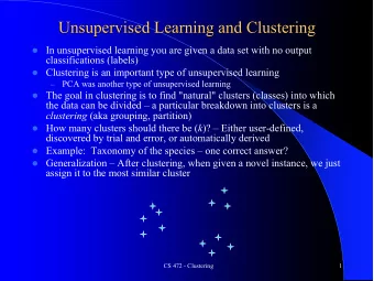
Returning to clustering… • Clusters may overlap • Some clusters may be “wider” than others • Can we model this explicitly? • With what probability is a point from a cluster?

ProbabilisMc Clustering • Try a probabilisMc model! Y X 1 X 2 • allows overlaps, clusters of different size, etc. ?? 0.1 2.1 • Can tell a genera*ve story for ?? 0.5 -1.1 data ?? 0.0 3.0 – P(Y)P(X|Y) ?? -0.1 -2.0 • Challenge: we need to esMmate ?? 0.2 1.5 model parameters without labeled Ys … … …

Gaussian Mixture Models • P(Y): There are k components • P(X|Y): Each component generates data from a mul>variate Gaussian with mean μ i and covariance matrix Σ i Each data point assumed to have been sampled from a genera4ve process : 1. Choose component i with probability P(y=i) [Mul*nomial] 2. Generate datapoint ~ N( m i , Σ i ) P ( X = x j | Y = i ) = µ 2 µ 1 T Σ i 1 1/ 2 exp − 1 ⎡ ⎤ − 1 x j − µ i ( ) ( ) 2 x j − µ i (2 π ) m / 2 || Σ i || ⎢ ⎥ ⎣ ⎦ By fi:ng this model (unsupervised µ 3 learning), we can learn new insights about the data

MulMvariate Gaussians # T Σ i & (2 π ) m /2 || Σ i || 1/2 exp − 1 1 − 1 x j − µ i P(X= x j )= ( ) ( ) P ( X = x j | Y = i ) = 2 x j − µ i % ( $ ' Σ ∝ idenMty matrix

MulMvariate Gaussians # T Σ i & (2 π ) m /2 || Σ i || 1/2 exp − 1 1 − 1 x j − µ i P(X= x j )= ( ) ( ) P ( X = x j | Y = i ) = 2 x j − µ i % ( $ ' Σ = diagonal matrix X i are independent ala Gaussian NB

MulMvariate Gaussians # T Σ i & (2 π ) m /2 || Σ i || 1/2 exp − 1 1 − 1 x j − µ i P(X= x j )= ( ) ( ) P ( X = x j | Y = i ) = 2 x j − µ i % ( $ ' Σ = arbitrary (semidefinite) matrix: - specifies rotaMon (change of basis) - eigenvalues specify relaMve elongaMon

MulMvariate Gaussians Eigenvalue, λ, of Σ Covariance matrix, Σ, = degree to which x i vary together # T Σ i & (2 π ) m /2 || Σ i || 1/2 exp − 1 1 − 1 x j − µ i P(X= x j )= ( ) ( ) P ( X = x j | Y = i ) = 2 x j − µ i % ( $ '

Modelling erupMon of geysers Old Faithful Data Set Time to ErupMon DuraMon of Last ErupMon

Modelling erupMon of geysers Old Faithful Data Set Single Gaussian Mixture of two Gaussians

Marginal distribuMon for mixtures of Gaussians Component Mixing coefficient K=3

Marginal distribuMon for mixtures of Gaussians

Learning mixtures of Gaussians Original data (hypothesized) Observed data (y missing) Inferred y’s (learned model) Shown is the posterior probability that a point was generated from i th Gaussian: Pr( Y = i | x )

ML esMmaMon in supervised setng • Univariate Gaussian • Mixture of Mul4 variate Gaussians ML esMmate for each of the MulMvariate Gaussians is given by: n µ ML = 1 n Σ ML = 1 k ∑ T k k x n k ∑ ( ) x j − µ ML ( ) x j − µ ML n n j = 1 j = 1 Just sums over x generated from the k ’th Gaussian

What about with unobserved data? • Maximize marginal likelihood : K – argmax θ ∏ j P(x j ) = argmax ∏ j ∑ k=1 P(Y j =k, x j ) • Almost always a hard problem! – Usually no closed form soluMon – Even when lgP(X,Y) is convex, lgP(X) generally isn’t… – Many local opMma

ExpectaMon MaximizaMon 1977: Dempster, Laird, & Rubin

The EM Algorithm • A clever method for maximizing marginal likelihood: – argmax θ ∏ j P(x j ) = argmax θ ∏ j ∑ k=1 K P(Y j =k, x j ) – Based on coordinate descent. Easy to implement (eg, no line search, learning rates, etc.) • Alternate between two steps: – Compute an expectaMon – Compute a maximizaMon • Not magic: s4ll op4mizing a non-convex func4on with lots of local op4ma – The computaMons are just easier (oZen, significantly so)

EM: Two Easy Steps Objec>ve: argmax θ lg ∏ j ∑ k=1 K P(Y j =k, x j ; θ) = ∑ j lg ∑ k=1 K P(Y j =k, x j ; θ) Data: {x j | j=1 .. n} • E-step : Compute expectaMons to “fill in” missing y values according to current parameters, θ – For all examples j and values k for Y j , compute: P(Y j =k | x j ; θ) • M-step : Re-esMmate the parameters with “weighted” MLE esMmates – Set θ new = argmax θ ∑ j ∑ k P(Y j =k | x j ;θ old ) log P(Y j =k, x j ; θ) Par>cularly useful when the E and M steps have closed form solu>ons

Gaussian Mixture Example: Start

AZer first iteraMon

AZer 2nd iteraMon

AZer 3rd iteraMon

AZer 4th iteraMon

AZer 5th iteraMon

AZer 6th iteraMon

AZer 20th iteraMon

EM for GMMs: only learning means (1D) Iterate: On the t ’th iteraMon let our esMmates be (t) } λ t = { μ 1 (t) , μ 2 (t) … μ K E-step Compute “expected” classes of all datapoints ⎛ ⎞ ) ∝ exp − 1 ( ( ) 2 σ 2 ( x j − µ k ) 2 P Y j = k x j , µ 1 ... µ K P Y j = k ⎜ ⎟ ⎝ ⎠ M-step Compute most likely new μ s given class expectaMons m ( ) ∑ P Y j = k x j x j j = 1 µ k = m ( ) ∑ P Y j = k x j j = 1

What if we do hard assignments? Iterate: On the t ’th iteraMon let our esMmates be (t) } λ t = { μ 1 (t) , μ 2 (t) … μ K E-step Compute “expected” classes of all datapoints ⎛ ⎞ ) ∝ exp − 1 ( ( ) 2 σ 2 ( x j − µ k ) 2 P Y j = k x j , µ 1 ... µ K P Y j = k ⎜ ⎟ ⎝ ⎠ M-step δ represents hard assignment to “most Compute most likely new μ s given class expectaMons likely” or nearest cluster m ( ) ∑ P Y j = k x j x j m ( ) x j ∑ δ Y j = k , x j j = 1 j = 1 µ k = µ k = m m ( ) ( ) ∑ ∑ δ Y j = k , x j P Y j = k x j j = 1 j = 1 Equivalent to k-means clustering algorithm!!!

E.M. for General GMMs p k (t) is shorthand for esMmate of P(y=k) on Iterate: On the t ’th iteraMon let our esMmates be t’th iteraMon λ t = { μ 1 (t) , μ 2 (t) … μ K (t) , Σ 1 (t) , Σ 2 (t) … Σ K (t) , p 1 (t) , p 2 (t) … p K (t) } E-step Compute “expected” classes of all datapoints for each class ( ) ∝ p k ( ) ( t ) p x j ; µ k ( t ) , Σ k ( t ) Evaluate probability of a P Y j = k x j ; λ t mul*variate a Gaussian at x j M-step Compute weighted MLE for μ given expected classes above T ( ) ( ) [ ] x j − µ k [ ] ∑ ∑ ( t + 1 ) ( t + 1 ) P Y j = k x j ; λ t x j P Y j = k x j ; λ t x j − µ k ) = ) = ( t + 1 j ( j t + 1 µ k Σ k ( ) ( ) ∑ ∑ P Y j = k x j ; λ t P Y j = k x j ; λ t j j ( ) ∑ P Y j = k x j ; λ t ( t + 1) = j p k m m = #training examples

The general learning problem with missing data • Marginal likelihood: X is observed, Z (e.g. the class labels Y ) is missing: • ObjecMve: Find argmax θ l(θ:Data) • Assuming hidden variables are missing completely at random (otherwise, we should explicitly model why the values are missing)