Unsupervised Learning and Inverse Problems with Deep Neural - PowerPoint PPT Presentation

Unsupervised Learning and Inverse Problems with Deep Neural Networks J oan Bruna, Stéphane Mallat, Ivan Dokmanic, Martin de Hoop École Normale Supérieure www.di.ens.fr/data

Deep Convolutional Networks ρ Φ ( x ) x ( u ) ρ L j L 1 f M ( x ) ρ ( u ) is a scalar non-linearity: max( u, 0) or | u | or ... Part III Inverse problems

Dimensionality Reduction Multiscale Interactions de d variables x ( u ): pixels, particules, agents... u 1 u 2

Deep Convolutional Trees ρ Φ ( x ) x ( u ) ρ L j y = ˜ f ( x ) L 1 L J Cascade of convolutions: no channel connections

Scale separation with Wavelets • Wavelet filter ψ ( u ): ψ 2 j , θ ( u ) = 2 − j ψ (2 − j r θ u ) rotated and dilated: ω 2 | ˆ ψ λ ( ω ) | 2 real parts imaginary parts ω 1 Z x ? 2 j , θ ( u ) = x ( v ) 2 j , θ ( u − v ) dv ✓ x ? � 2 J ( u ) ◆ : average • Wavelet transform: Wx = x ? 2 j , θ ( u ) : higher j ≤ J, θ frequencies Preserves norm: � Wx � 2 = � x � 2 .

Fast Wavelet Filter Bank 2 0 | W 1 | 2 1 | x ? 2 1 , θ | 2 J Scale

Wavelet Filter Bank x ( u ) 2 0 ρ ( α ) = | α | | W 1 | | W 1 | 2 1 | x ? 2 1 , θ | 2 2 | x ? 2 2 , θ | | x ? 2 j , θ | 2 J Scale

Wavelet Scattering Network 2 0 x ρ L 1 2 1 ρ L 2 | x ? λ 1 | ρ L J 2 J || x ? λ 1 | ? λ 2 | ? � J x ? � J Scale ρ W 1 ρ W 2 ... ρ W J S J = n o ||| x ? λ 1 | ? λ 2 ? ... | ? λ m | ? � J S J x = ρ ( α ) = | α | λ k Interactions across scales

Scattering Properties   x ? � 2 J | x ? λ 1 | ? � 2 J   = . . . | W 3 | | W 2 | | W 1 | x   || x ? λ 1 | ? λ 2 | ? � 2 J S J x =     ||| x ? λ 2 | ? λ 2 | ? λ 3 | ? � 2 J   ... λ 1 , λ 2 , λ 3 ,... k | W k x | � | W k x 0 | k  k x � x 0 k k W k x k = k x k ) Lemma : k [ W k , D τ ] k = k W k D τ � D τ W k k  C kr τ k ∞ Theorem : For appropriate wavelets, a scattering is contractive k S J x � S J y k  k x � y k ( L 2 stability ) preserves norms k S J x k = k x k translations invariance and deformation stability: if D τ x ( u ) = x ( u − τ ( u )) then J →∞ k S J D τ x � S J x k  C kr τ k ∞ k x k lim

Digit Classification: MNIST Joan Bruna Supervised y = f ( x ) S J x x Linear classifier Invariants to specific deformations Invariants to translations Separates di ff erent patterns Linearises small deformations No learning Classification Errors Training size Conv. Net. Scattering 50000 0 . 4% 0 . 4% LeCun et. al.

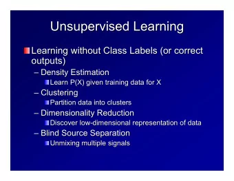
Part II- Unsupervised Learning Unsupervised learning: Approximate the probability distribution p ( x ) of X ∈ R d given P realisations { x i } i ≤ P with potentially P = 1

Stationary Processes   X ? � 2 J ( t ) | X ? λ 1 | ? � 2 J ( t )   : stationary vector   || X ? λ 1 | ? λ 2 | ? � 2 J ( t ) S J X =     ||| X ? λ 2 | ? λ 2 | ? λ 3 | ? � 2 J ( t )   ... λ 1 , λ 2 , λ 3 ,...

Ergodicity and Moments Central limit theorem with ”weak” ergodicity conditions   E ( X ) E ( | X ? λ 1 | )     E ( SX ) = E ( || X ? λ 1 | ? λ 2 | )     E ( ||| X ? λ 2 | ? λ 2 | ? λ 3 | )   ... λ 1 , λ 2 , λ 3 ,...

Generation of Random Processes • Reconstruction: compute ˜ X which satisfies with random initialisation and gradient descent.

Texture Reconstructions Joan Bruna Ising-critical Turbulence 2D

Representation of Audio Textures Joan Bruna Gaussian Original in time 60 ω 20 40 Applauds 60 t 20 Paper 40 60 Cocktail Party

Max Entropy Canonical Models • A representation Φ ( x ) = { φ k ( x ) } k ≤ K with x ∈ R d Z µ k = E ( φ k X ) = φ k ( x ) p ( x ) dx R maximum entropy: H ( p ) = − p ( x ) log p ( x ) dx p ( x ) = Z − 1 exp ⇣ ⌘ X θ k φ k ( x ) ⇒ − k

Ergodic Microcanonical Model R d

Uniform Distribution on Balls d | x ( k ) | 2 ⌘ 1 / 2 ⇣ X Φ x = d − 1 / 2 k x k 2 = • Sphere in R d d − 1 = µ k =1 d X • Simplex in R d Φ x = d − 1 k x k 1 = d − 1 | x ( k ) | = µ k =1

Scattering Representation • Scattering coe ffi cients of order 0, 1 and 2: n o d − 1 X x ( u ) , d − 1 k x ? λ 1 k 1 , d − 1 k | x ? λ 1 | ? λ 2 k 1 Φ x = u

Microcanonical Scattering R d

Scattering Approximations ˜ X µ = E ( Φ X ) X If

Ergodic Microcanonical Model R d

Singular Ergodic Processes

Scattering Ising

Stochastic Geometry: Cox Process

Non-Ergodic Mixture R d

Non-Ergodic Microcanonical Mixture R d

Scattering Multifractal Processes • Scattering coe ffi cients of order 0, 1 and 2:

Scat Ising at Critical Temperature

Failures of Audio Synthesis J. Anden and V. Lostanlen Time Scattering Original

Time-Frequency Translation Group J. Anden and V. Lostanlen Time-frequency wavelet convolutions t log λ t t t t || x ? λ | ? α ? β | ? � J | x ? λ | ? � J

Joint Time-Frequency Scattering J. Anden and V. Lostanlen Time Scattering Time/Freq Scattering Original

Part III- Supervised Learning x J ( u, k J ) x 2 ( u, k 2 ) x ( u ) x 1 ( u, k 1 ) ρ L J classification ρ L 1 k 1 k 2 x j = ρ L j x j − 1 • L j is a linear combination of convolutions and subsampling: ⇣ X ⌘ x j ( u, k j ) = ⇢ x j − 1 ( · , k ) ? h k j ,k ( u ) k sum across channels What is the role of channel connections ?

Environmental Sound Classification J. Anden and V. Lostanlen Supervised y = f ( x ) S J x x Linear classifier No learning UrbanSound8k: 10 classes air conditioner car horns 8k training examples class-wise average error MFCC audio descriptors 0,39 children playing dog barks time scattering 0,27 drilling engine at idle ConvNet 
 0,26 (Piczak, MLSP 2015) time-frequency scattering 0,2

Inverse Scattering Transform Joan Bruna • Given S J x we want to compute ˜ x such that:     x ? � 2 J x ? � 2 J ˜ | ˜ x ? λ 1 | ? � 2 J | x ? λ 1 | ? � 2 J = S J x     S J ˜ x = =     ... ...     ||| ˜ x ? λ 1 | ? .. | ? λ m | ? � 2 J ||| x ? λ 1 | ? .. | ? λ m | ? � 2 J λ 1 ,..., λ m λ 1 ,..., λ m We shall use m = 2. • If x ( u ) is a Dirac, or a straight edge or a sinusoid then ˜ x is equal to x up to a translation.

Sparse Shape Reconstruction Joan Bruna With a gradient descent algorithm: Original images of N 2 pixels: m = 1, 2 J = N : reconstruction from O (log 2 N ) scattering coe ff . m = 2, 2 J = N : reconstruction from O (log 2 2 N ) scattering coe ff .

Multiscale Scattering Reconstructions Original Images N 2 pixels Scattering Reconstruction 2 J = 16 1 . 4 N 2 coe ff . 2 J = 32 0 . 5 N 2 coe ff . 2 J = 64 2 J = 128 = N

III- Inverse Problems F x y • Best Linear Method: Least Squares estimate (linear interpolation): y = ( b x b Σ † ˆ Σ xy ) x

Super-Resolution F x y •Best Linear Method: Least Squares estimate (linear interpolation): y = ( b x b Σ † •State-of-the-art Methods: ˆ Σ xy ) x – Dictionary-learning Super-Resolution – CNN-based: Just train a CNN to regress from low-res to high- res. – They optimize cleverly a fundamentally unstable metric criterion: Θ ∗ = arg min k F ( x i , Θ ) � y i k 2 , ˆ X y = F ( x, Θ ∗ ) Θ i

Scattering Super-Resolution x y F S L − α ,J x S L,J x   x ? � 2 J ( u ) | x ? j 1 ,k 1 | ? � 2 J ( u ) S L,J x =   || x ? j 1 ,k 1 | ? j 2 ,k 2 | ? � 2 J ( u ) L ≤ j 1 ,j 2 ≤ J • Linear estimation in the scattering domain • No phase estimation: potentially worst PSNR • Good image quality because of deformation stability


 Super-Resolution Results J. Bruna, P. Sprechmann Linear Estimate Original state-of-the-art Scattering

Super-Resolution Results J. Bruna, P. Sprechmann Best 
 Scattering 
 Original state-of-the-art Linear Estimate Estimate

Super-Resolution Results J. Bruna, P. Sprechmann Best 
 Scattering 
 Original state-of-the-art Linear Estimate Estimate

Super-Resolution Results I. Dokmanic, J. Bruna, M. De Hoop l 1 Regularization Original A TV Regularization Original Scattering Scattering Low-Resolution Low-Resolution

Tomography Results I. Dokmanic, J. Bruna, M. De Hoop B C TV Regularization Original Scattering Low-Resolution

Conclusions • Deep convolutional networks have spectacular high-dimensional and generic approximation capabilities. • New stochastic models of images for inverse problems. • Outstanding mathematical problem to understand deep nets: – How to learn representations for inverse problems ? Understanding Deep Convolutional Networks , arXiv 2016.