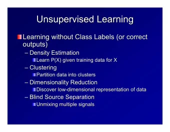
Unsupervised Learning About this class Build a model for your data. - PowerPoint PPT Presentation

Unsupervised Learning About this class Build a model for your data. Which datapoints Unsupervised learning are similar? k -means Clustering Nowadays lots of work on using unlabeled data to improve the performance of supervised learn- Expectation Maximization ing 1 2

k -means Clustering Problem: given m data points, break them up into k clusters, where k is pre-specified x i ∈ C j || x i − µ j || 2 Objective: minimize � k � Always terminates at a local minimum j =1 where µ j is the cluster mean Bad clustering examples for k = 2 (circles) and k = 3 (bad initialization leads to bad results) Algorithm: Issues with k -means: how to choose k and how Initialize µ 1 , . . . , µ k randomly to initialize Repeat until convergence: Possible ideas: Use multiple runs with di ff er- ent random start configurations? Pick starting 1. Assign each x i to the cluster with the clos- points far apart from each other? est mean 2. Calculate the new mean for each cluster 1 � µ j ← x i | C j | x i ∈ C j 3

Assume the two Gaussians have the same vari- Expectation Maximization ance σ and unknown means µ 1 and µ 2 . What are the maximum likelihood estimates of µ 1 (EM developed by Dempster, Rubin & Laird, and µ 2 ? 1977. These notes mostly from Tom Mitchell’s book, with some other references thrown in for How do we think about this problem? Start good measure) by thinking about each data point as a tuple ( x i , z i 1 , z i 2 ) where the z s indicate which of the Let’s do away with the “hard” assignments and distributions the points were drawn from (but maximize data likelihood! they are unobserved). Suppose points on the real line are drawn from Now apply the EM algorithm. Start with arbi- one of two Gaussian distributions using the fol- trary values for µ 1 and µ 2 . Now repeat until lowing algorithm: we have converged to stationary values for µ 1 and µ 2 : 1. One of the two Gaussians is selected 1. Compute each expected value E [ z ij ] as- 2. A point is sampled from the selected Gaus- suming the means of the Gaussians are ac- sian and placed on the real line tually the current estimates of µ 1 and µ 2 4

EM in General Define: f ( x = x i | µ = µ 1 ) E [ z i 1 ] = 1. θ : parameters governing the data (what f ( x = x i | µ = µ 1 ) + f ( x = x i | µ = µ 2 ) we’re trying to find ML estimates of exp( − 1 2 σ 2 ( x i − µ 1 ) 2 ) = exp( − 1 2 σ 2 ( x i − µ 1 ) 2 ) + exp( − 1 2 σ 2 ( x i − µ 2 ) 2 ) 2. X : observed data 2. Compute updated (maximum likelihood) es- 3. Z : unobserved data timates of µ 1 and µ 2 using the expected values E [ z ij ] from step 1. 4. Y = X ∪ Z � m i =1 E [ z ij ] x i µ i = � m i =1 E [ z ij ] We want to find ˆ θ that maximizes E [ln Pr( Y | θ )] The expectation is taken because Y itself is a random variable (the Z part is unknown!) 5

But we don’t know the distribution governing Y , so how do we take the expecation? EM uses the current estimate of θ , call it h , to estimate the distribution governing Y Define Q ( h ′ | h ) that gives the expected log prob- 2. Maximization (M) step: Replace h by the ability above, assuming that the data were gen- h ′ that maximizes Q erated by h Q ( h ′ | h ) = E [ln Pr( Y | h ′ ) | h, X ] Again, only guaranteed to converge to a local minimum Now EM consists of repeating the next two steps until convergence 1. Estimation (E) step: Calculate Q ( h ′ | h ) us- ing the current estimate h and the observed data X to estimate the probability distribu- tion over Y

Deriving Mixtures of Gaussians And the expectation of z ij is computed as be- fore, based on the current hypothesis : Let’s do this for k Gaussians exp( − 1 2 σ 2 ( x i − µ j ) 2 ) E [ z ij ] = n =1 exp( − 1 � k 2 σ 2 ( x i − µ n ) 2 ) First, let’s derive an expression for Q ( h ′ | h ) E-step defines the Q -function in terms of the expectations generated by the previous esti- k 2 πσ 2 exp( − 1 1 j ) 2 f ( y i | h ′ ) = � z ij ( x i − µ ′ √ mate. 2 σ 2 j =1 Then the M-step chooses a new estimate to maximize the Q -function, which is equivalent   m m k 1 1 to finding the µ ′ j ) 2 j that minimize: � ln f ( y i | h ′ ) = � � z ij ( x i − µ ′  ln √ 2 πσ 2 −  2 σ 2 i =1 i =1 j =1 m k j ) 2 � � E [ z ij ]( x i − µ ′ Taking the expectation and using E [ f ( z )] = i =1 j =1 f ( E [ z ]) when f is linear: This is just a maximum likelihood problem with the solution described earlier, namely:   � m m k i =1 E [ z ij ] x i 1 1 j ) 2 Q ( h ′ | h ) = � � E [ z ij ]( x i − µ ′  ln √ 2 πσ 2 − � m  2 σ 2 i =1 E [ z ij ] i =1 j =1 6