Uncertainty Outside and Inside Economic Models Nobel Lecture Lars - PowerPoint PPT Presentation
Uncertainty Outside and Inside Economic Models Nobel Lecture Lars Peter Hansen University of Chicago December 8, 2013 1 / 22 Skepticism Le doute nest pas une condition agr eable, mais la certitude est absurde. Voltaire (1776) 2 / 22
Uncertainty Outside and Inside Economic Models Nobel Lecture Lars Peter Hansen University of Chicago December 8, 2013 1 / 22
Skepticism Le doute n’est pas une condition agr ´ eable, mais la certitude est absurde. Voltaire (1776) 2 / 22
Components of Uncertainty ◮ Risk - probabilities assigned by a given model ◮ Ambiguity - not knowing which among a family of models should be used to assess risk Skepticism about the model specification 3 / 22
Researcher and Investor Uncertainty ◮ Researchers outside a model Given a dynamic economic model: ◮ estimate unknown parameters; ◮ assess model implications. ◮ Investors inside a model In constructing a dynamic economic model: ◮ depict economic agents (consumers, enterprises, policy makers) as they cope with uncertainty; ◮ construct equilibrium interactions that acknowledge this uncertainty. 4 / 22
Overview: Techniques and Applications ◮ Time series econometrics and rational expectations ◮ Generalized Method of Moments estimation, applications and extensions ◮ Empirical challenges ◮ Uncertainty and investors inside the model ◮ Uncertainty and policy 5 / 22
Time Series Econometrics and Rational Expectations ◮ Bachelier (1901) - Slutsky (1926) -Yule (1927): random shocks are impulses for time series. ◮ finance ◮ macroeconomics ◮ Frisch (1933) - Haavelmo (1943): dynamic models provide a formal connection between economic inputs and statistical methods used outside the model. ◮ Muth (1961) - Lucas (1972): economic agents inside the model have rational expectations. 6 / 22
Rational Expectations Econometrics ◮ Expectations determined inside the model. ◮ A new form of econometric restrictions. ◮ Challenge: Requires a complete model specification including a specification of the information available to the economic agents inside the model. Early work by Sargent (1973) and others, and my initial publication Hansen and Sargent (1980). 7 / 22
Doing Something without Doing Everything ◮ Generalized Method of Moments estimation ◮ Study partially specified models that link financial markets and the macroeconomy. ◮ Build and extend an earlier econometrics literature on estimating equations in a simultaneous system, in particular Sargan (1958, 1959). 8 / 22
Doing Something without Doing Everything Model the investment in risky capital and the pricing of financial assets: � �� S t + ℓ � � � � E X t + ℓ � F t = Q t S t where ◮ S is a stochastic discount factor (SDF) process; ◮ X t + ℓ vector of payoffs on physical or financial assets; ◮ ℓ is the investment horizon; ◮ Q t vector of asset prices; ◮ F t is the investor information; ◮ E is the expectation implied by the data generating process and used by investors inside the model . 9 / 22
Doing Something without Doing Everything ◮ Recall � �� S t + ℓ � � � � E X t + ℓ − Q t � F t = 0 . S t ◮ Z t : variables in the investor information set F t . Then �� S t + ℓ � � E X t + ℓ Z t − Q t Z t = 0 . S t Observations: ◮ SDF depends on data and model parameters; ◮ Approximate expectations by time series averages; ◮ Build and justify formal methods for estimation and inference; ◮ Avoid a complete specification of investor information; ◮ Extend to other applications: estimate and assess misspecified models. 10 / 22
Further Econometric Challenges ◮ Formal study of an entire class of estimators: ◮ pose as a semi-parametric estimation problem; ◮ construct a well defined efficiency bound for the class of the many possible estimators. Hansen (1985) and Chamberlain (1987) ◮ Related approaches: ◮ Ignore parametric representation of the SDF. Empirical pricing restrictions are consistent with many SDF’s. Hansen and Jaganathan (1991), Luttmer (1996) ◮ SDF model misspecified. A different perspective on estimation and model comparison. Hansen and Jaganathan (1997), Hansen, Heaton and Luttmer (1995) 11 / 22
Applications to Empirical Finance Hansen and co-authors ◮ Hodrick (1980,1983) - characterizing risk premia in forward foreign exchange market; ◮ Singleton (1982,1983) - macro finance linkages implied by the SDF for macroeconomists’ “typical” model of investors; ◮ Richard (1987) - conditioning information and risk -return tradeoffs given a “general specification” of SDFs; ◮ Jagannathan (1991) and Cochrane (1992) - empirical characterizations of SDF’s without parametric restrictions. Jagannathan Hodrick Singleton Richard Cochrane 12 / 22
The Changing Price of Uncertainty Stochastic discount factors encode compensations for exposure to risk: risk prices. Finding: “risk price” channel provides a predictable and important source for variation observed in security markets. ◮ SDF’s are highly variable. ◮ Volatility is conditional on information pertinent to investors. ◮ Volatility is higher in bad macroeconomic times than good ones. Campbell-Cochrane (1999). Modeling challenge : What is the source of this SDF volatility? Possible explanation : Investor concern about misspecification inside a dynamic economic model. 13 / 22
Asset Pricing under a Belief Distortion �� � � � � � S t + ℓ � � E X t + ℓ � � F t = Q t (1) � S t where � E is the distorted expectation operator and � S is the corresponding stochastic discount factor. ◮ Convenient to represent distorted beliefs using a positive martingale M with a unit expectation via the formula: �� M t + ℓ � � � � � � E [ Y t + ℓ |F t ] = E Y t + ℓ � F t . M t ◮ Rewrite (1) as: �� � � � � �� S t + ℓ � � � M t + ℓ � � S t + ℓ � � E X t + ℓ � F t � = E X t + ℓ � F t = Q t M t � S t S t where S = M � S . 14 / 22
Asset Pricing under a Belief Distortion SDF representation � S = M S distorted risk beliefs preferences ◮ � S constructed from data and model parameters. ◮ M is a likelihood ratio. ◮ When M close to one, the distortion is small. ◮ Statistical criteria provide interpretable measures of the magnitude of the distortion. When the distortion is small, a statistician with a large number of observations will struggle to tell the difference between two models. 15 / 22
Statistical Quantification as a Guide for Modeling � S = M S distorted risk beliefs preference Statistical tools support a refinement of rational expectations ( M = 1). ◮ Inspiration: detect when historical evidence is less informative; ◮ Discipline: limit the scope of belief distortions such as: ◮ animal spirits ◮ heterogeneous beliefs ◮ subjective concerns about rare events ◮ overconfidence 16 / 22
Modeling Challenges � S = M S distorted risk beliefs preference ◮ Challenges: ◮ Add structure and content to belief distortions. ◮ Make the belief distortions a formal source for fluctuating uncertainty prices. ◮ Approach: model misspecification and uncertainty more broadly conceived. 17 / 22
C o m p o ne nts of U ncert ai nty R o b ust ness: a f a mil y Π a n d e x pl ore utility c o nse q ue nces of ( 1 9 5 4) S a v a ge ( 1 9 3 7) de Fi netti ( 1 9 3 9) W al d ( 1 9 2 1) K ni g ht m o del a ver a ge . alter n ati ve π ’s. I m ple me nte d by a dist orte d φ ( |x , θ)π (d θ ) Ris k: a distri b uti o n f or ne xt p eri o ds o utc o me Y φ ( |x ) = ¯ m o dels. Re d ucti o n: a u ni q ue π a n d a ver a ge o ver a f a mil y Π of pr o b a bility distri b uti o ns π o ver θ . A m bi g uity: de nsity φ ( |x , θ). i n de xe d by a p ar a meter θ . Re prese nt as a p eri o ds st ate X gi ve n t his 1 8 / 2 2
Operationalizing Robustness and Ambiguity Aversion Conceptual apparatus: ◮ Explore a family of perturbations to a model subject to constraints or penalization. (Origins in control theory) ◮ Explore a family of “posteriors/priors” used to weight models. Dynamic and robust extension of Bayesian decision theory. (Origins in statistics) What is available: ◮ Extensions of Savage’s axiomatic foundations. ◮ Tractable representations. 19 / 22
Enriching the Uncertainty Pricing Dynamics ◮ Two reasons for skepticism about models: ◮ some future model variations cannot be inferred from past evidence; ◮ while some features of models can be inferred from past evidence there remains prior ambiguity. ◮ Outcome: Uncertainty in the persistence of macroeconomic growth. High persistence is bad in bad times and low persistence is bad in good times. This becomes a source for ex post distortions in beliefs and uncertainty prices that change over time in interesting ways. ◮ Explicit model of M and thus S that depends on macroeconomic shocks, state vector and model parameters where: � S = M S distorted risk beliefs preference 20 / 22
Uncertainty and Policy Implications Two approaches ◮ Uncertainty outside structural econometric models; ◮ Equilibrium interactions within a model when policy makers and the private sector simultaneously confront uncertainty. 21 / 22
Implications for Financial Oversight ◮ Systemic risk: a grab bag of scenarios rationalizing interventions in financial markets. ◮ Haldane (Bank of England), Tarullo (Board of Governors): Limited understanding of systemic risk challenges its value as a guiding principle for financial oversight! ◮ Systemic uncertainty ◮ Complicated problems do not necessarily require complicated solutions. 22 / 22
Recommend
More recommend
Explore More Topics
Stay informed with curated content and fresh updates.
