Uncertainty Analysis for Linear Parameter Varying Systems Peter - PowerPoint PPT Presentation
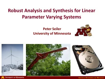
Aerospace Engineering and Mechanics Uncertainty Analysis for Linear Parameter Varying Systems Peter Seiler Department of Aerospace Engineering and Mechanics University of Minnesota Joint work with: H. Pfifer, T. P eni (Sztaki), S. Wang, G.
Aerospace Engineering and Mechanics Uncertainty Analysis for Linear Parameter Varying Systems Peter Seiler Department of Aerospace Engineering and Mechanics University of Minnesota Joint work with: H. Pfifer, T. P´ eni (Sztaki), S. Wang, G. Balas, A. Packard (UCB), and A. Hjartarson (MuSyn) Research supported by: NSF (NSF-CMMI-1254129), NASA (NRA NNX12AM55A), and Air Force Office of Scientific Research (FA9550-12-0339) 1
Aerospace Engineering and Mechanics Aeroservoelastic Systems Objective: Enable lighter, more efficient aircraft by active control of aeroelastic modes. Boeing: 787 Dreamliner http://www.uav.aem.umn.edu/ AFLR/Lockheed/NASA: BFF and X56 MUTT 2
Aerospace Engineering and Mechanics Supercavitating Vehicles Objective: Increase vehicle speed by traveling within the cavitation bubble. Ref: D. Escobar, G. Balas, and R. Arndt, ”Planing Avoidance Control for Supercavitating Vehicles,” ACC, 2014. 3
Aerospace Engineering and Mechanics Wind Turbines Objective: Increase power capture, decrease structural loads, and enable wind to provide ancillary services. http://www.eolos.umn.edu/ Clipper Turbine at Minnesota Eolos Facility 4
Aerospace Engineering and Mechanics Wind Turbines Objective: Increase power capture, decrease structural loads, and enable wind to provide ancillary services. Clipper Turbine at Minnesota Eolos Facility http://www.eolos.umn.edu/ 5
Aerospace Engineering and Mechanics Outline Goal: Synthesize and analyze controllers for these systems. 1 Linear Parameter Varying (LPV) Systems 2 Uncertainty Modeling with IQCs 3 Robustness Analysis for LPV Systems 4 Connection between Time and Frequency Domain 5 Summary 6
Aerospace Engineering and Mechanics Outline Goal: Synthesize and analyze controllers for these systems. 1 Linear Parameter Varying (LPV) Systems 2 Uncertainty Modeling with IQCs 3 Robustness Analysis for LPV Systems 4 Connection between Time and Frequency Domain 5 Summary 7
Aerospace Engineering and Mechanics Parameterized Trim Points These applications can be described by nonlinear models: x ( t ) = f ( x ( t ) , u ( t ) , ρ ( t )) ˙ y ( t ) = h ( x ( t ) , u ( t ) , ρ ( t )) where ρ is a vector of measurable, exogenous signals. Assume there are trim points (¯ x ( ρ ) , ¯ u ( ρ ) , ¯ y ( ρ )) parameterized by ρ : 0 = f (¯ x ( ρ ) , ¯ u ( ρ ) , ρ ) y ( ρ ) = h (¯ ¯ x ( ρ ) , ¯ u ( ρ ) , ρ ) 8
Aerospace Engineering and Mechanics Linearization Let ( x ( t ) , u ( t ) , y ( t ) , ρ ( t )) denote a solution to the nonlinear system and define perturbed quantities: δ x ( t ) := x ( t ) − ¯ x ( ρ ( t )) δ u ( t ) := u ( t ) − ¯ u ( ρ ( t )) δ y ( t ) := y ( t ) − ¯ y ( ρ ( t )) Linearize around (¯ x ( ρ ( t )) , ¯ u ( ρ ( t )) , ¯ y ( ρ ( t )) , ρ ( t )) ˙ δ x = A ( ρ ) δ x + B ( ρ ) δ u + ∆ f ( δ x , δ u , ρ ) − ˙ x ( ρ ) ¯ ˙ δ y = C ( ρ ) δ x + D ( ρ ) δ u + ∆ h ( δ x , δ u , ρ ) where A ( ρ ) := ∂f ∂x (¯ x ( ρ ) , ¯ u ( ρ ) , ρ ) , etc. 9
Aerospace Engineering and Mechanics LPV Systems This yields a linear parameter-varying (LPV) model: ˙ δ x = A ( ρ ) δ x + B ( ρ ) δ u + ∆ f ( δ x , δ u , ρ ) − ˙ x ( ρ ) ¯ ˙ δ y = C ( ρ ) δ x + D ( ρ ) δ u + ∆ h ( δ x , δ u , ρ ) Comments: • LPV theory a extension of classical gain-scheduling used in industry, e.g. flight controls. • Large body of literature in 90’s: Shamma, Rugh, Athans, Leith, Leithead, Packard, Scherer, Wu, Gahinet, Apkarian, and many others. • − ˙ x ( ρ ) can be retained as a measurable disturbance. ¯ • Higher order terms ∆ f and ∆ h can be treated as memoryless, nonlinear uncertainties. 10
Aerospace Engineering and Mechanics Grid-based LPV Systems x ( t ) = A ( ρ ( t )) x ( t ) + B ( ρ ( t )) d ( t ) ˙ e ( t ) = C ( ρ ( t )) x ( t ) + D ( ρ ( t )) d ( t ) Parameter vector ρ lies within a set of admissible trajectories A := { ρ : R + → R n ρ : ρ ( t ) ∈ P , ˙ ρ ( t ) ∈ ˙ P ∀ t ≥ 0 } Grid based LPV systems LFT based LPV systems ρI e d G ρ e d G (Pfifer, Seiler, ACC, 2014) (Scherer, Kose, TAC, 2012) 11
Aerospace Engineering and Mechanics Outline Goal: Synthesize and analyze controllers for these systems. 1 Linear Parameter Varying (LPV) Systems 2 Uncertainty Modeling with IQCs 3 Robustness Analysis for LPV Systems 4 Connection between Time and Frequency Domain 5 Summary 12
Aerospace Engineering and Mechanics Integral Quadratic Constraints (IQCs) z Ψ v w ∆ Let Ψ be a stable, LTI system and M a constant matrix. Def.: ∆ satisfies IQC defined by Ψ and M if � T z ( t ) T Mz ( t ) dt ≥ 0 0 for all v ∈ L 2 [0 , ∞ ) , w = ∆( v ) , and T ≥ 0 . (Megretski, Rantzer, TAC, 1997) 13
Aerospace Engineering and Mechanics Example: Memoryless Nonlinearity w = ∆( v, t ) is a memoryless nonlinearity in the sector [ α, β ] . v w ∆ 2( βv ( t ) − w ( t ))( w ( t ) − αv ( t )) ≥ 0 ∀ t 14
Aerospace Engineering and Mechanics Example: Memoryless Nonlinearity w = ∆( v, t ) is a memoryless nonlinearity in the sector [ α, β ] . v w ∆ 2( βv ( t ) − w ( t ))( w ( t ) − αv ( t )) ≥ 0 ∀ t � ∗ � − 2 αβ � v ( t ) α + β � � v ( t ) � ≥ 0 ∀ t w ( t ) α + β − 2 w ( t ) Pointwise quadratic constraint 14
Aerospace Engineering and Mechanics Example: Norm Bounded Uncertainty ∆ is a causal, SISO operator with � ∆ � ≤ 1 . � w � ≤ � v � v w ∆ 15
Aerospace Engineering and Mechanics Example: Norm Bounded Uncertainty ∆ is a causal, SISO operator with � ∆ � ≤ 1 . � w � ≤ � v � v w ∆ � ∞ � T � 1 � v ( t ) � � v ( t ) � 0 dt ≥ 0 w ( t ) 0 − 1 w ( t ) 0 for all v ∈ L 2 [0 , ∞ ) and w = ∆( v ) . Infinite time horizon constraint 15
Aerospace Engineering and Mechanics Example: Norm Bounded Uncertainty ∆ is a causal, SISO operator with � ∆ � ≤ 1 . � w � ≤ � v � v w ∆ � T � T � 1 � v ( t ) � � v ( t ) � 0 dt ≥ 0 w ( t ) 0 − 1 w ( t ) 0 for all v ∈ L 2 [0 , ∞ ) , w = ∆( v ) , and T ≥ 0 Causality implies finite-time constraint. 16
Aerospace Engineering and Mechanics Example: Norm Bounded Uncertainty ∆ causal with � ∆ � ≤ 1 � T � T � 1 � v ( t ) � � v ( t ) � 0 dt ≥ 0 w ( t ) 0 − 1 w ( t ) 0 ∀ v ∈ L 2 [0 , ∞ ) and w = ∆( v ) . v w ∆ 17
Aerospace Engineering and Mechanics Example: Norm Bounded Uncertainty ∆ causal with � ∆ � ≤ 1 � T � 1 � 0 z ( t ) T z ( t ) dt ≥ 0 z 0 − 1 I 0 ∀ v ∈ L 2 [0 , ∞ ) and w = ∆( v ) . v w ∆ 17
Aerospace Engineering and Mechanics Example: Norm Bounded Uncertainty ∆ causal with � ∆ � ≤ 1 � T z ( t ) T Mz ( t ) dt ≥ 0 z Ψ 0 ∀ v ∈ L 2 [0 , ∞ ) and w = ∆( v ) . v w ∆ ∆ satisfies IQC defined by � 1 � 0 Ψ = I 2 and M = 0 − 1 17
Aerospace Engineering and Mechanics Example: Norm Bounded LTI Uncertainty ∆ is LTI and � ∆ � ≤ 1 z Ψ For any stable system D , ∆ satisfies v w IQC defined by ∆ � D � � 1 � 0 0 Ψ = and M = 0 D 0 − 1 � T z ( t ) T Mz ( t ) dt ≥ 0 Equivalent to D -scales in 0 µ -analysis 18
Aerospace Engineering and Mechanics IQCs in the Time Domain z Ψ v w ∆ Let Ψ be a stable, LTI system and M a constant matrix. Def.: ∆ satisfies IQC defined by Ψ and M if � T z ( t ) T Mz ( t ) dt ≥ 0 0 for all v ∈ L 2 [0 , ∞ ) , w = ∆( v ) , and T ≥ 0 . (Megretski, Rantzer, TAC, 1997) 19
Aerospace Engineering and Mechanics Outline Goal: Synthesize and analyze controllers for these systems. 1 Linear Parameter Varying (LPV) Systems 2 Uncertainty Modeling with IQCs 3 Robustness Analysis for LPV Systems 4 Connection between Time and Frequency Domain 5 Summary 20
Aerospace Engineering and Mechanics Background Nominal Performance of LPV Systems Induced L 2 gain: � e � � G ρ � = sup � d � d � =0 ,d ∈ L 2 ,ρ ∈A ,x (0)=0 Bounded Real Lemma like condition to compute upper bound (Wu, Packard, ACC 1995) 21
Aerospace Engineering and Mechanics Background Nominal Performance of LPV Integral Quadratic Constraints Systems • general framework for robustness analysis Induced L 2 gain: • originally in the frequency domain � e � • known LTI system under � G ρ � = sup � d � perturbations d � =0 ,d ∈ L 2 ,ρ ∈A ,x (0)=0 ∆ Bounded Real Lemma like v w condition to compute upper bound e G d (Wu, Packard, ACC 1995) (Megretski, Rantzer, TAC, 1997) 21
Aerospace Engineering and Mechanics Worst-case Gain • Goal: Assess stability and performance for the interconnection of known LPV system G ρ and “perturbation” ∆ . ∆ v w G ρ e d 22
Aerospace Engineering and Mechanics Worst-case Gain • Goal: Assess stability and performance for the interconnection of known LPV system G ρ and “perturbation” ∆ . ∆ • Approach: Use IQCs to specify a v w finite time horizon constraint on the G ρ input/output behavior of ∆ . e d 22
Recommend
More recommend
Explore More Topics
Stay informed with curated content and fresh updates.
