Types of Environments Goal Based Agents Plan ahead Fully - PDF document

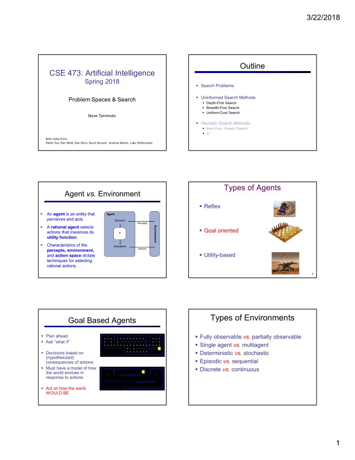
3/22/2018 Outline CSE 473: Artificial Intelligence Spring 2018  Search Problems  Uninformed Search Methods Problem Spaces & Search  Depth-First Search  Breadth-First Search  Uniform-Cost Search Steve Tanimoto  Heuristic Search Methods  Best-First, Greedy Search  A* With slides from : Dieter Fox, Dan Weld, Dan Klein, Stuart Russell, Andrew Moore, Luke Zettlemoyer Types of Agents Agent vs. Environment  Reflex  An agent is an entity that Agent perceives and acts . Sensors Percepts  A rational agent selects Environment  Goal oriented actions that maximize its ? utility function .  Characteristics of the Actuators percepts, environment, Actions  Utility-based and action space dictate techniques for selecting rational actions. 4 Types of Environments Goal Based Agents  Plan ahead  Fully observable vs. partially observable  Ask “what if”  Single agent vs. multiagent  Deterministic vs. stochastic  Decisions based on (hypothesized)  Episodic vs. sequential consequences of actions  Must have a model of how  Discrete vs. continuous the world evolves in response to actions  Act on how the world WOULD BE 1

3/22/2018 Example: Traveling in Romania Search thru a Problem Space (aka State Space) Problem Space (aka State Space) • Input:  State space:  Set of states  Cities  Operators [and costs]  Successor function:  Start state  Roads: Go to adjacent city with cost = distance  Goal state [test]  Start state:  Arad • Output:  Goal test: • Path: start a state satisfying goal test  Is state == Bucharest? [May require shortest path]  Solution? [Sometimes just need a state that passes test] Example: Simplified Pac-Man State Space Sizes?  Input:  Search Problem:  A state space Eat all of the food  Pacman positions: 10 x 12 = 120 10 x 12 = 120  A successor function “N”, 1.0  Pacman facing: up, down, left, right up, down, left, right  Food configurations: 2 30 2 30 “E”, 1.0  A start state  Ghost1 positions: 12 12  Ghost 2 positions: 11 11  A goal test  Output: 120 x 4 x 2 30 x 12 x 11 = 6.8 x 10 13 State Space Graphs Search Trees This is now / start  State space graph: “N”, 1.0 “E”, 1.0  Each node is a state G a  The successor function is c b Possible futures represented by arcs e  Edges may be labeled with d f costs S h  In a search graph, each state p r  A search tree: occurs only once! q  Start state at the root node  We can rarely build this graph Ridiculously tiny search graph  Children correspond to successors in memory (so we don’t) for a tiny search problem  Nodes contain states, correspond to PLANS to those states  Edges are labeled with actions and costs  For most problems, we can never actually build the whole tree 2

3/22/2018 State Space Graphs vs. Search Trees State Space Graphs vs. Search Trees Consider this 4-state How big is its search tree Each NODE in State Space graph: (from S)? Search Tree in the search Graph tree is an S entire PATH in the state G e p a a d space graph. c b e h r q b c e G S d f a a h r p q f S We construct h q c p q f G both on b p r q demand – and a q c G we construct a as little as possible. Important: Lots of repeated structure in the search tree! Tree Search Search Example: Romania Searching with a Search Tree General Tree Search  Important ideas:  Search:  Fringe  Expand out potential plans (tree nodes)  Expansion  Maintain a fringe of partial plans under  Exploration strategy consideration  Main question: which fringe nodes to explore?  Try to expand as few tree nodes as possible 3

3/22/2018 Tree Search Example Depth-First Search G a c b e d f S h p r q Depth-First Search Depth-First Search G G a Strategy: expand a a a Strategy: expand a c c c deepest node first b deepest node first b b e e e Implementation: Fringe is Implementation: Fringe is d d d f f f a LIFO stack S a LIFO stack S h h h p r p p r r q q q S e p d q b c e h r a a h r p q f q c p q f G a q c G a Search Algorithm Properties Search Algorithm Properties  Complete: Guaranteed to find a solution if one exists?  Optimal: Guaranteed to find the least cost path?  Time complexity? 1 node  Space complexity? b b nodes … b 2 nodes  Cartoon of search tree: m tiers  b is the branching factor  m is the maximum depth  solutions at various depths b m nodes  Number of nodes in entire tree?  1 + b + b 2 + …. b m = O(b m ) 4

3/22/2018 Depth-First Search (DFS) Properties Breadth-First Search  What nodes does DFS expand? 1 node  Some left prefix of the tree. b b nodes …  Could process the whole tree! b 2 nodes  If m is finite, takes time O(b m ) m tiers  How much space does the fringe take?  Only has siblings on path to root, so O(bm) b m nodes  Is it complete?  m could be infinite, so only if we prevent cycles  Is it optimal?  No, it finds the “leftmost” solution, regardless of depth or cost Breadth-First Search Breadth-First Search (BFS) Properties  What nodes does BFS expand? a G Strategy: expand a c b shallowest node first  Processes all nodes above shallowest solution 1 node e b Implementation: Fringe d  Let depth of shallowest solution be d f b nodes … is a FIFO queue S h d tiers  Search takes time O(b d ) b 2 nodes p r q  How much space does the fringe take? b d nodes S  Has roughly the last tier, so O(b d ) e p d  Is it complete? b m nodes Search q b c e h r  d must be finite if a solution exists, so yes! Tiers a a h r p q f  Is it optimal? q c  Only if costs are all 1 (more on costs later) p q f G a q c G a DFS vs BFS Memory a Limitation?  Suppose: • 4 GHz CPU • 32 GB main memory • 100 instructions / expansion • 5 bytes / node • 40 M expansions / sec • Memory filled in 160 sec … 3 min Algorithm Complete Optimal Time Space DFS w/ Path N unless N O( b m ) O( bm ) Checking finite BFS Y Y O( b d ) O( b d ) 5

3/22/2018 Iterative Deepening BFS vs. Iterative Deepening Iterative deepening uses DFS as a subroutine: b  For b = 10, d = 5: … 1. Do a DFS which only searches for paths of length 1 or less. 2. If “1” failed, do a DFS which only searches paths  BFS = 1 + 10 + 100 + 1,000 + 10,000 + 100,000 = of length 2 or less. 111,111 3. If “2” failed, do a DFS which only searches paths of length 3 or less.  IDS = 6 + 50 + 400 + 3,000 + 20,000 + 100,000 = ….and so on. 123,456 Algorithm Complete Optimal Time Space w/ Path DFS  Overhead = (123,456 - 111,111) / 111,111 = 11% Y N O( b m ) O( bm ) Checking BFS Y Y O( b d ) O( b d ) ID Y Y O( b d ) O( bd )  Memory BFS: 100,000; IDS: 50 32 Costs on Actions Uniform Cost Search Expand GOAL a 2 2 cheapest c b 3 node first: GOAL 2 a 2 2 1 8 Fringe is a 2 e c b 3 3 d 2 priority f 1 8 9 8 2 queue 2 e START h 3 d 4 1 1 f 9 8 2 4 p r 15 START h q 4 1 1 4 p 15 r Notice that BFS finds the shortest path in terms of number of q transitions. It does not find the least-cost path. Uniform Cost Search (UCS) Uniform Cost Search Properties 2 G a Strategy: expand a  What nodes does UCS expand? c b 1 8 cheapest node first: 2 2  Processes all nodes with cost less than cheapest solution! e 3 b d f 9 8 2  If that solution costs C* and arcs cost at least ε , then the “effective C ≤ 1 Fringe is a priority … S h 1 depth” is roughly C*/ε queue (priority: C ≤ 2 C*/ε 1 p r cumulative cost)  Takes time O(b C*/ε ) (exponential in effective depth) q “tiers” 15 C ≤ 3  How much space does the fringe take? 0 S  Has roughly the last tier, so O(b C*/ε ) e 9 p 1 d 3  Is it complete? 11 q 16 4 e 5 h 17 r b c 11  Assuming best solution has a finite cost and minimum arc cost is positive, yes! Cost a 6 a h 13 r 7 p q f contours  Is it optimal? q c p q f 8 G  Yes! a q 11 c 10 G a 6

3/22/2018 Uniform Cost Search Uniform Cost Search Algorithm Complete Optimal Time Space  Strategy: expand lowest … c  1 DFS w/ Path path cost Y N O( b m ) O( bm ) Checking c  2 BFS Y Y O( b d ) O( b d ) c  3  The good: UCS is UCS Y* Y O( b C*/ε ) O( b C*/ε ) complete and optimal! b  The bad: …  Explores options in every C*/ ε tiers “direction”  No information about goal location Start Goal Uniform Cost: Pac-Man The One Queue  All these search algorithms  Cost of 1 for each action are the same except for  Explores all of the states, but one fringe strategies  Conceptually, all fringes are priority queues (i.e. collections of nodes with attached priorities)  Practically, for DFS and BFS, you can avoid the log(n) overhead from an actual priority queue, by using stacks and queues  Can even code one implementation that takes a variable queuing object To Do:  Look at the course website:  http://http://courses.cs.washington.edu/courses/cse473/18sp/  Do the readings (Ch 3)  Do Project 0 if new to Python  Start Project 1. 7