Bayesian Variable Selection via Spike-and-Slab Priors: Annotated - PDF document

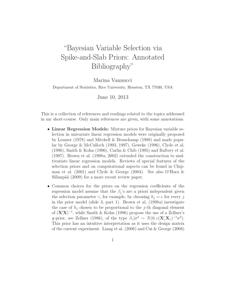
“Bayesian Variable Selection via Spike-and-Slab Priors: Annotated Bibliography” Marina Vannucci Department of Statistics, Rice University, Houston, TX 77030, USA June 10, 2013 This is a collection of references and readings related to the topics addressed in my short-course. Only main references are given, with some annotations. • Linear Regression Models: Mixture priors for Bayesian variable se- lection in univariate linear regression models were originally proposed by Leamer (1978) and Mitchell & Beauchamp (1988) and made popu- lar by George & McCulloch (1993, 1997), Geweke (1996), Clyde et al. (1996), Smith & Kohn (1996), Carlin & Chib (1995) and Raftery et al. (1997). Brown et al. (1998 a , 2002) extended the construction to mul- tivariate linear regression models. Reviews of special features of the selection priors and on computational aspects can be found in Chip- man et al. (2001) and Clyde & George (2004). See also O’Hara & Sillanp¨ a¨ a (2009) for a more recent review paper. • Common choices for the priors on the regression coefficients of the regression model assume that the β j ’s are a priori independent given the selection parameter γ , for example, by choosing h j = c for every j in the prior model (slide 3, part 1). Brown et al. (1998 a ) investigate the case of h j chosen to be proportional to the j -th diagonal element of ( X ′ X ) − 1 , while Smith & Kohn (1996) propose the use of a Zellner’s g -prior, see Zellner (1986), of the type β γ | σ 2 ∼ N (0 , c ( X ′ γ X γ ) − 1 σ 2 ). This prior has an intuitive interpretation as it uses the design matrix of the current experiment. Liang et al. (2008) and Cui & George (2008) 1

have investigated formulations that use a fully Bayesian approach by imposing mixtures of g-priors on c . They also propose hyper-g priors for c which leads to closed form marginal likelihoods and nonlinear shrinkage via Empirical Bayes procedures. • Independent Bernoulli priors on the γ j ’s with a Beta hyperprior, w ∼ Beta ( a, b ), with a, b to be chosen, are used for example by Brown et al. (1998 b ). An attractive feature of these priors is that appropriate choices of w that depend on p impose an a priori multiplicity penalty, as argued in Scott & Berger (2010). Applications of Bayesian variable selection models to the analysis of genomic data have looked into priors on γ that exploit the complex dependence structure between genes (variables) as captured via underlying biological processes and/or networks. Some of these contributions include Li & Zhang (2010) and Stingo et al. (2010, 2011). • When a large number of predictors makes the full exploration of the model space unfeasible, Monte Carlo Markov chain methods can be used as stochastic searches to quickly and efficiently explore the poste- rior distribution looking for “good” models, i.e., models with high pos- terior probability, see George & McCulloch (1997). The most popular is the Metropolis scheme (MC 3 ), proposed by Madigan & York (1995) in the context of model selection for discrete graphical models and sub- sequently adapted to variable selection, see Raftery et al. (1997) and Brown et al. (1998 b , 2002), among others. Improved MCMC schemes have been proposed to achieve an even faster exploration of the poste- rior space, see for example the shotgun algorithm of Hans et al. (2007) and the evolutionary Monte Carlo schemes combined with parallel tem- pering proposed by Bottolo & Richardson (2010), Bottolo et al. (2011) (software available at http://www.bgx.org.uk/software.html). • Variable selection can be achieved by thresholding marginal posterior probabilities of inclusion. Barbieri & Berger (2004) define the median- probability model, which is the model that includes those covariates having posterior inclusion probability at least 1/2, and show that, under many circumstances, this model has greater predictive power than the most probable. Another method chooses a cut-off threshold based on the expected false discovery rate, see Newton et al. (2004). 2

• Extensions to Probit and Logit Models: The prior models for vari- able selection described above can be easily applied to other modeling settings, where a response variable is expressed as a linear combinations of the predictors. For example, Bayesian variable selection for probit models is investigated by Sha et al. (2004) and Kwon et al. (2007), within the data augmentation framework of Albert & Chib (1993). Holmes & Held (2006) (with correction in Bayesian Analysis (2011), 6(2) ) and T¨ uchler (2008) considered logistic models - see also Polson & Scott (2013) for an alternative data augmentation scheme. Gustafson & Lefebvre (2008) extended methodologies to settings where the subset of predictors associated with the propensity to belong to a class varies with the class. Sha et al. (2006) considered accelerated failure time models for survival data. • Generalized Linear Models: Probit and logit models, in particular, belong to the more general class of generalized linear models (GLMs) of McCullagh & Nelder (1989), that assume the distribution of the response variable as coming from the exponential family. Conditional densities in the general GLM framework cannot be obtained directly and the resulting mixture posterior may be difficult to sample using standard MCMC methods due to multimodality. Some attempts to Bayesian variable selection methods for GLMs were done by Raftery (1996), who proposed approximate Bayes factors, and by Ntzoufras et al. (2003), who developed a method to jointly select variables and the link function. See also Ibrahim et al. (2000) and Chen et al. (2003). • Covariance Selection in Models with Random Effects: Among possible extensions of linear models, we also mention the class of mixed models, that include random effects capturing heterogeneity among subjects, Laird & Ware (1982). One challenge in developing SSVS ap- proaches for random effects models is the constraint that the random effects covariance matrix needs to be semi-definite positive. Chen & Dunson (2003) imposed mixture priors on the regression coefficients of the fixed effects and achieve simultaneous selection of the random effects by imposing variable selection priors on the components in a special LDU decomposition of the random effects covariance. A simi- lar approach, based on the Cholesky decomposition, was proposed by Fr¨ uhwirth-Schnatter & T¨ uchler (2008). Cai & Dunson (2006) extended 3

the approach to generalized linear mixed models (GLMM) and Kinney & Dunson (2007) to logistic mixed effects models for binary data. Fi- nally, MacLehose et al. (2007), Dunson et al. (2008) and Yang (2012) considered Bayesian nonparametric approaches that use spiked Dirich- let process priors. Their approach models the unknown distribution of the regression coefficients via a Dirichlet process prior with a spike- and-slab centering distribution. This allows different predictors to have identical coefficients while performing variable selection. There, the clustering induced by the Dirichlet process is on the univariate regres- sion coefficients and strength is borrowed across covariates. Kim et al. (2010) consider similar priors in a random effects model to cluster the coefficient vectors across samples. • Regularization Priors: With spike and slab priors, all possible mod- els are embodied within a hierarchical formulation and variable selec- tion is carried out model-wise. Regularization approaches, instead, use priors with just one continuous component and rely on the shrinkage properties of Bayesian estimators. Examples include the Laplace prior and the ridge prior. These have a singularity at the origin, which pro- motes an intensive shrinkage towards the zero prior mean. These priors can be expressed as scale mixture of normal distributions to facilitate computation. Popular regularized regression techniques include the Bayesian LASSO of Park & Casella (2008) and Hans (2009), which is equivalent to the MAP estimation under normal/exponential (Laplace) prior, and the normal scale mixture priors proposed of Griffin & Brown (2010). Li & Lin (2010) proposed the elastic net, which encourages a grouping effect in which strongly correlated predictors tend to come in or out of the model together. Lasso procedures tend to overshrink large coefficients due to the relatively light tails of the Laplace prior. To over- come the issue, Carvalho et al. (2010) and Armagan et al. (2013) have proposed the horseshoe prior and generalized double Pareto shrinkage prior for linear models, respectively. The posterior summary measures (mean or median) are never zero with a positive probability, and zeroing the redundant variables out then needs to be carried out via threshold- ing the estimated coefficients. A solution is to augment the shrinkage priors to include a point mass at zero, see for example Hans (2010). • Mixture Models: Bayesian variable selection has been applied also to 4