Two views of Duality: Lagrangians and Geometric 1 Linear Programs. - PDF document

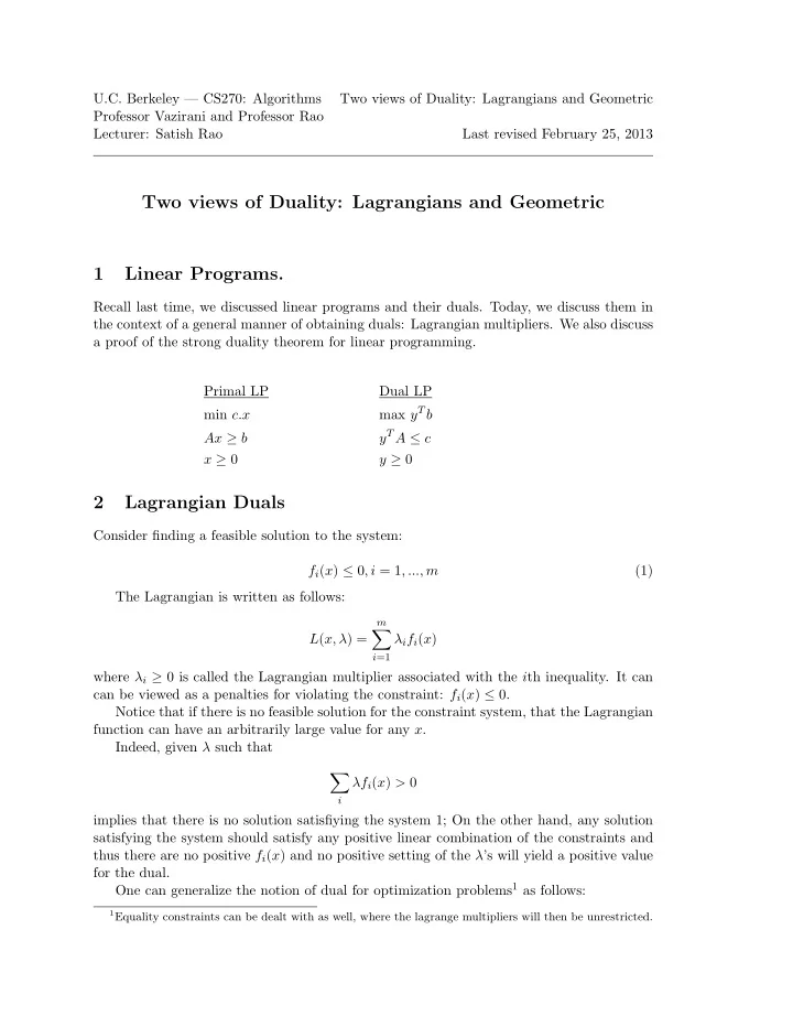
U.C. Berkeley — CS270: Algorithms Two views of Duality: Lagrangians and Geometric Professor Vazirani and Professor Rao Lecturer: Satish Rao Last revised February 25, 2013 Two views of Duality: Lagrangians and Geometric 1 Linear Programs. Recall last time, we discussed linear programs and their duals. Today, we discuss them in the context of a general manner of obtaining duals: Lagrangian multipliers. We also discuss a proof of the strong duality theorem for linear programming. Primal LP Dual LP max y T b min c.x y T A ≤ c Ax ≥ b x ≥ 0 y ≥ 0 2 Lagrangian Duals Consider finding a feasible solution to the system: f i ( x ) ≤ 0 , i = 1 , ..., m (1) The Lagrangian is written as follows: m � L ( x, λ ) = λ i f i ( x ) i =1 where λ i ≥ 0 is called the Lagrangian multiplier associated with the i th inequality. It can can be viewed as a penalties for violating the constraint: f i ( x ) ≤ 0. Notice that if there is no feasible solution for the constraint system, that the Lagrangian function can have an arbitrarily large value for any x . Indeed, given λ such that � λf i ( x ) > 0 i implies that there is no solution satisfiying the system 1; On the other hand, any solution satisfying the system should satisfy any positive linear combination of the constraints and thus there are no positive f i ( x ) and no positive setting of the λ ’s will yield a positive value for the dual. One can generalize the notion of dual for optimization problems 1 as follows: 1 Equality constraints can be dealt with as well, where the lagrange multipliers will then be unrestricted.

2 Notes for Two views of Duality: Lagrangians and Geometric: min f ( x ) (2) subject to f i ( x ) ≤ 0 , i = 1 , ..., m (3) (4) The corresponding Lagrangian function will be m � L ( x, λ ) = f ( x ) + λ i f i ( x ) i =1 Here, in the case that there is a feasible primal solution with value v , the dual solution can only have nonzero values for λ i > 0 with f i ( x ) = 0 . Moreover, the value of the best λ will also be v . We can also see that if there is a λ where for all x , L ( x, λ ) ≥ α , that the value of the minimization function for problem 2 is at least α ; the optimal feasible solution for 2 yields this value for any dual value of λ. The primal problem is to find an x that maximizes the Lagrange function over any value of the dual. For convex programs, these values will be the same. For any setup the dual provides a lower bound on the optimal solution of the primal. It is often used in that manner as a heuristic approach to solving constrained optimization problems. 2.1 Linear Program. For a linear program, we have min c · x subject to b i − a i · x ≤ 0 , i = 1 , ..., m And a Lagrangian formulation of � λ i ( b i − a i x i ) . 2 L ( λ, x ) = cx + i We can rewrite the function as follows: � L ( λ, x ) = − ( x j ( a j λ − c j )) + bλ. j Translating back to a set of linear inequalities one gets the following problem. max b · λ 2 Note for any x , the minimizing λ can only take nonzero values for i where ( b i − a i x i ) is zero. This is the complementary slackness condition that we discussed before in the context of linear programs.

3 Notes for Two views of Duality: Lagrangians and Geometric: x p b Figure 1: ( p − x ) T ( b − p ) < 0 for x in convex body. a j · λ ≤ c j . The linear programming dual of 5! That is the Lagrangian dual problem, of finding a lower bound for the Langrangian function for any x , is the linear programming dual. Again, this technique applies more generally, but it is informative to see that this for- mulation is equivalent to the linear programming. One might surmise that the nice part of the problem may behave nicely with this formulation. 3 Strong Duality We will begin a discussion of a the proof of strong duality here. We saw a proof based on experts for the special case of zero sum 2 person games. We discuss a geometric proof here. We begin with the notion of that a convex bodies can be separated using a hyperplane. We refer the student to a proof of of Farkas lemma and then finally prove a version of LP duality at http://www-math.mit.edu/ goemans/18415/18415-FALL01/lect9-19.ps 3.1 Convex Separator. Theorem 1 For any convex body A , and a point b , either b ∈ A or there exists a point where ( p − x ) t ( b − p ) ≤ 0 . Proof: Choose p as the closest point in A to b in the convex region. For the sake of contradition, there is an x ∈ A , where ( x − p ) T ( b − p ) > 0. For some intuition, note that the angle between ( x − p ) and ( b − p ) is less than 90. Since A is convex every point between p and x is in A . Moreover, there must be a point closer to b along this path. Again some intution. In the figure below, a portion of the line segment between p and x is inside the circle of radius | p − b | , and thus there is a closer point to b along this line segment. This contradicts that p is the closest point in A to p . p p b x To prove this formally, one can express the squared distance to b of a point p + ( x − p ) µ as

4 Notes for Two views of Duality: Lagrangians and Geometric: ( | p − b | − µ | x − p | cosθ ) 2 + ( µ | x − p | sinθ ) 2 where θ is the angle between x − p and b − p . (See the figure below.) | p − b | − ℓcosθ p ℓcosθ b θ ℓsinθ ℓ = µ | x − p | Distance to new point. p + µ ( x − p ) x Simplifying (and substituting that sin 2 θ = (1 − cos 2 θ ), we obtain the following?: | p − b | 2 − 2 µ | p − b || x − p | cosθ + ( µ | x − p | ) 2 . Taking the derivative with respect to µ yields, − 2 | p − b || x − p | cosθ + 2( µ | x − p | ) . which is negative for a small enough value of µ ( for positive cosθ. ) End of proof. 3.2 Convex to Strong Duality. We refer the reader to www-math.mit.edu/ goemans/18415/18415-FALL01/lect9-19.ps. (The proof there is does not have so much intuition. But it does do a translation from the simple geometric lemma above.) What one should get from this picture is that there is a translation of the problem of solving an LP back and forth from the problem of finding a separating hyperplane for a convex region from a point. The notion that there is a separating hyperplane follows from finding the point in the convex region that is “closest” to b . One could proceed by identifying a closer point to b . This problem turns out to be finding a positive solution to a single linear equation; i.e., a dot product is positive. Thus, again, as with experts and the Lagrangian dual, one sees that satisfying many constraints can be approached by iteratively satisfying a linear combination of those constraints.